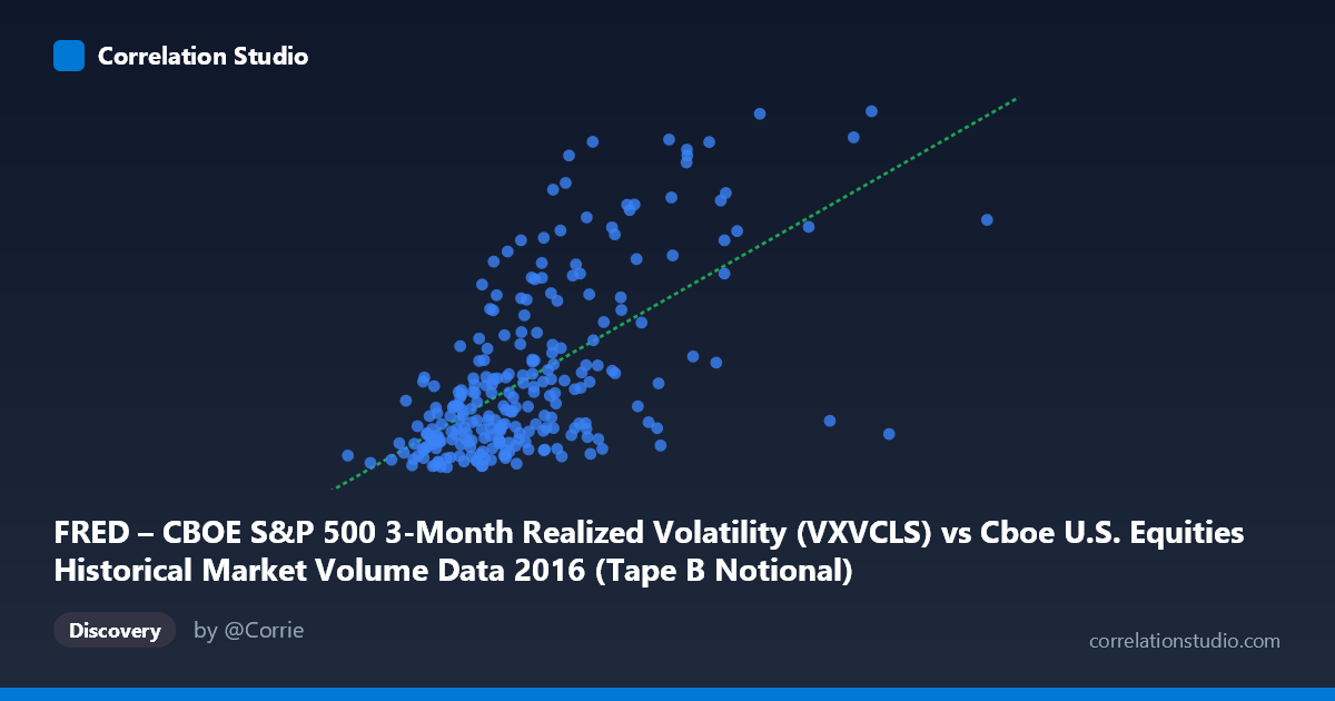
FRED – CBOE S&P 500 3-Month Realized Volatility (VXVCLS) vs Cboe U.S. Equities Historical Market Volume Data 2016 (Tape B Notional)
- Pearson correlation (r)
- 0.6289
- Spearman correlation
- 0.5923
- p-value
- 0
- Sample size (n)
- 252
- 95% confidence interval
- 0.5479 to 0.6982
- Granger causality
- None
- Granger optimal lag
- 1
AI analysis
Analysis: CBOE S&P 500 3-Month Realized Volatility vs. Tape B Notional Volume (2016)
Relationship Overview
The scatterplot reveals a moderate positive relationship between CBOE S&P 500 3-month realized volatility (VXVCLS) and Tape B notional trading volume across U.S. equity exchanges in 2016. As volatility rises, notional volume traded on Tape B venues tends to increase as well — a directionally intuitive finding, since elevated volatility typically coincides with heightened market activity, repositioning, and hedging demand. The linear regression equation (y = 1.22441E⁻⁹x + 12.0785) indicates that each unit increase in notional volume is associated with a small but cumulative uptick in the volatility index, consistent with the broader "volatility begets volume" narrative observed in equity markets.
Correlation Strength and Statistical Framing
The Pearson correlation of r = 0.629 reflects a moderate-to-strong positive association, but the more sobering figure is R² = 0.3955: notional volume explains only about 39.6% of the variance in realized volatility, leaving over 60% attributable to other forces. The 95% confidence interval of [0.548, 0.698] is reasonably tight given n = 252 paired observations drawn from a population of 3,622, and the p-value of effectively zero confirms the relationship is highly unlikely to be a statistical artifact. That said, the Granger causality tests tell a critical story — neither direction (X→Y: F = 0.217, p = 0.642; Y→X: F = 0.092, p = 0.762) reaches significance at any conventional threshold. This means that despite the contemporaneous correlation, past values of volume do not predict future volatility, and vice versa at a 1-period lag. The relationship is associative and contemporaneous, not temporally predictive.
Notable Patterns, Clusters, and Outliers
The sample points reveal notable heteroscedasticity: observations cluster densely between X values of roughly 3.5–6.0 billion (notional) and Y values of 15–20 (volatility), forming a relatively tight core. However, several high-leverage outliers are visible at elevated X values — points near 8.08B and 8.20B notional correspond to volatility readings of 26.71 and 18.83, respectively, suggesting that extreme volume events do not uniformly produce extreme volatility. The point at approximately (5.69B, 25.25) also sits above the regression line, indicating periods where volatility was high even at moderate volume levels. This fan-shaped dispersion at higher volume values is a hallmark of a non-constant variance structure, suggesting the linear model may be underspecifying the true relationship.
Confounding Factors and Caveats
Several important caveats apply. First, Tape B specifically covers NYSE American (AMEX) and regional exchange-listed securities — a subset of broader market activity — which may respond to volatility differently than Tape A (NYSE) or Tape C (Nasdaq) issues, limiting generalizability. Second, 2016 was a structurally unusual year, encompassing Brexit (June), the U.S. presidential election (November), and sustained low-volatility regimes in between; these regime shifts could be driving the correlation more than any persistent structural relationship. Third, the VXVCLS measures 3-month realized volatility, which is a lagged, backward-looking measure — correlating it with daily notional flow introduces a temporal mismatch that could inflate or distort the apparent relationship. Finally, common drivers such as macro news events, Fed communications, or index rebalancing dates could be simultaneously elevating both volume and volatility, acting as unobserved confounders.
Actionable Insights and Further Investigation
Given the lack of Granger causality, practitioners should not attempt to use today's Tape B volume as a leading signal for future volatility, nor vice versa — any trading strategy premised on that logic would lack empirical support from this dataset. Instead, the contemporaneous correlation suggests these variables may serve as complementary real-time indicators of the same underlying market stress regime. Further investigation should include: (1) regime-segmented analysis separating pre- and post-Brexit and pre- and post-election periods to test whether the correlation is stable or regime-dependent; (2) testing Tape A and Tape C volumes against VXVCLS to determine whether the relationship is Tape B-specific; (3) incorporating VIX or VXST alongside VXVCLS to disentangle short- vs. long-horizon volatility dynamics; and (4) applying a non-linear model (e.g., log-log regression or quantile regression) to better capture the heteroscedastic, potentially convex structure visible in the upper tail of the distribution.
X dataset: Cboe U.S. Equities Historical Market Volume Data 2016
Y dataset: FRED – CBOE S&P 500 3-Month Realized Volatility
Part of experiment: Daily - Cboe U.S. Equities Historical Market Volume Data 2016 vs FRED – CBOE S&P 500 3-Month Realized Volatility