Datahub.io – WTI Daily Spot Price CSV (Price) vs Cboe U.S. Equities Historical Market Volume Data 2016 (Tape C Notional)
- Pearson correlation (r)
- -0.4293
- Spearman correlation
- -0.4228
- p-value
- 0
- Sample size (n)
- 252
- 95% confidence interval
- -0.525 to -0.3228
- Granger causality
- None
- Granger optimal lag
- 1
AI analysis
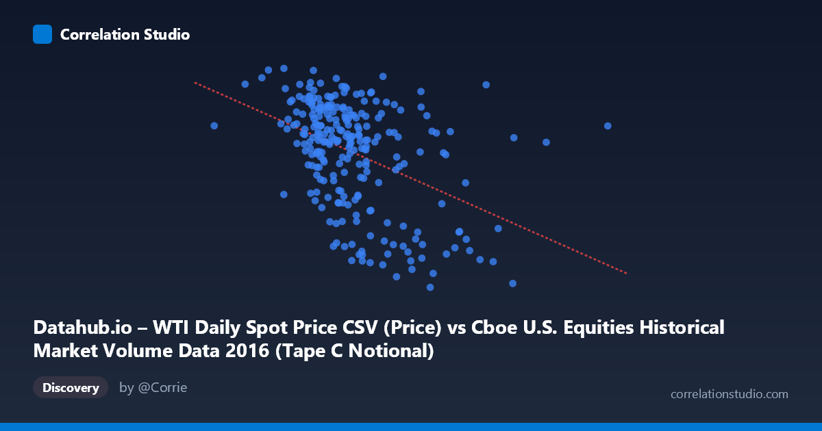
Scatterplot Analysis: WTI Oil Price vs. Cboe Tape C Notional Volume (2016)
Relationship Overview
The scatterplot reveals a moderate negative relationship between WTI daily spot oil prices (X-axis) and Cboe Tape C notional trading volume (Y-axis) across 2016 trading days. The linear regression equation (y = -2.54×10⁻⁹x + 55.94) confirms that as oil prices rise, Tape C notional volume tends to decline, and vice versa. Visually, the data cloud slopes downward from left to right, though with considerable scatter around the trend line. This suggests the relationship, while real, is embedded in a noisy, complex market environment where many other forces are simultaneously at work.
Correlation Strength and Statistical Significance
The Pearson correlation of r = -0.4293 indicates a moderate negative association, but the explained variance tells a more sobering story: r² = 0.1843 means only ~18.4% of the variance in Tape C notional volume is accounted for by WTI prices, leaving over 80% unexplained by this single variable. The 95% confidence interval of [-0.525, -0.323] is meaningfully away from zero and entirely negative, providing strong directional confidence. The p-value of 1.01×10⁻¹² is highly significant given the sample of 252 paired observations drawn from a population of 3,622, making it virtually certain this is not a chance correlation. However, Granger causality tests fail in both directions — neither X→Y (F=0.33, p=0.57) nor Y→X (F=0.48, p=0.49) reaches significance at a one-period lag — meaning that despite the contemporaneous correlation, neither variable reliably predicts the other's next-day movement. Correlation here is associative, not temporally predictive.
Notable Patterns, Clusters, and Outliers
Several structural features stand out in the data cloud. There is a visible cluster of points in the X range of roughly 4.0–5.5 billion (corresponding to lower-to-mid oil price regimes) where Tape C notional values are broadly distributed between ~38 and 54, suggesting high variability in equity volume even at similar oil price levels. At higher X values (above ~6.0 billion, i.e., elevated oil prices), points tend to pull toward lower Y values, reinforcing the negative trend — but a handful of notable outliers exist here with relatively high Tape C volume despite high oil prices (e.g., the point near 6,474 billion / 49.10 and 6,022 billion / 48.72), which resist the overall trend. At the lower end of the oil price range (below ~4.0 billion), Y values tend to be elevated, consistent with the negative slope. The sample statistics confirm a wide X range spanning nearly 8.7 billion units, while Y is more constrained (26–54), which means a few extreme X observations may be disproportionately influencing the regression slope.
Confounding Factors and Interpretive Caveats
The 2016 timeframe introduces important context: this period included significant macroeconomic events including OPEC production decisions, the U.S. presidential election, Brexit aftermath, and Federal Reserve rate movements — all of which simultaneously drove both oil prices and equity market activity in complex, non-linear ways. The axes are somewhat counterintuitively labeled (the dataset names appear swapped between axes — the WTI price column appears on the X-axis from a Cboe dataset, and the Tape C notional appears on the Y-axis from a WTI dataset), which warrants careful verification of data provenance before drawing conclusions. Additionally, Tape C notional volume reflects market activity in NYSE Arca-listed securities, which may have sector-specific exposure to energy prices, but this is a narrow slice of broader market dynamics. Common-cause confounding is highly plausible — a third variable such as market volatility (VIX), risk appetite, or economic surprise indices may be driving both oil prices and equity volumes simultaneously without a direct causal link between them.
Actionable Insights and Further Investigation
Despite modest explained variance, the statistically robust negative correlation warrants further exploration. A natural next step would be to test non-linear models (e.g., polynomial or spline regression) to check whether the relationship exhibits threshold effects — for instance, whether extreme oil price moves (crashes or spikes) produce outsized volume reactions. Incorporating VIX or realized volatility as a control variable would help isolate whether this correlation persists after accounting for the general market fear/uncertainty channel. The failed Granger causality at lag-1 suggests testing longer lags (2–5 days), as institutional responses to oil price moves may take several days to manifest in equity volumes. Finally, breaking the analysis by quarter or by sector exposure within Tape C would clarify whether the relationship is seasonal (oil in early 2016 was near multi-year lows and recovered sharply) or structurally persistent, which would significantly sharpen the practical interpretability of this finding.
X dataset: Cboe U.S. Equities Historical Market Volume Data 2016
Y dataset: Datahub.io – WTI Daily Spot Price CSV
Part of experiment: Daily - Cboe U.S. Equities Historical Market Volume Data 2016 vs Datahub.io – WTI Daily Spot Price CSV