Bitcoin Historical Data (2010-2024) (AssetEODCompletionTime) vs CryptoDataDownload – Binance BTC/USDT Daily OHLCV (High)
- Pearson correlation (r)
- 0.85
- Spearman correlation
- 0.886
- p-value
- 0
- Sample size (n)
- 3191
- 95% confidence interval
- 0.8401 to 0.8593
- Granger causality
- None
- Granger optimal lag
- 10
AI analysis
Analysis of BTC/USDT Timestamp vs. Price (High) Relationship
1. What the Visualization Reveals
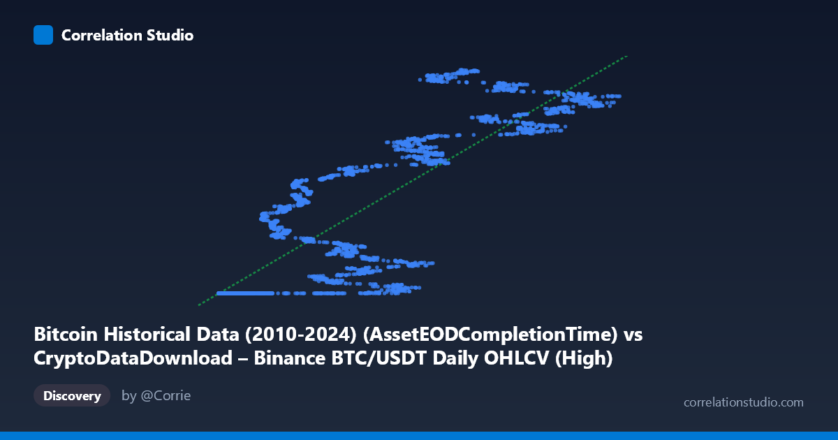
This scatterplot is somewhat unusual in that the "X" variable is actually a timestamp/completion-time field rather than a conventional independent variable — meaning this is effectively a time-series price chart of Bitcoin's daily high price, disguised as a correlation study. The data shows BTC's High price plotted against its own completion timestamp (encoded numerically), spanning 2017–2026. The pattern reveals distinct clustering: a large mass of points around X ≈ 3,000–20,000 sitting at a nearly flat Y-value (~1,614,337,000–1,614,338,000), followed by a scattered upward-trending cloud as X increases toward 60,000–126,000, where Y climbs to 1,660,000,000–1,780,000,000.
2. Strength, Direction, and Statistical Confidence
The correlation coefficient (r = 0.85) indicates a strong positive relationship, with R² = 0.7225 meaning roughly 72% of the variance in Y is statistically explained by X — a substantial but incomplete fit, leaving ~28% of variance unexplained by this linear model. The 95% CI [0.8401, 0.8593] is tight, and p ≈ 0 confirms this correlation is highly unlikely due to chance given the large sample (n=3,191). However, Granger causality testing shows no significant predictive direction in either direction (X→Y: p=0.31; Y→X: p=0.13). This is a critical caveat: despite strong contemporaneous correlation, neither variable helps forecast the other over time at the tested lag structure (10 periods). This strongly suggests the correlation is a structural/mechanical artifact (timestamp increasing alongside price over a bull-market period) rather than a genuine causal or forecastable relationship.
3. Notable Patterns and Non-Linearities
The chart is clearly non-linear and heteroscedastic. There's a dense horizontal band at low X values where Y is nearly constant (~1.614B) — likely representing an early period (2017-2018) where price was flat/low relative to later years, with many repeated near-identical values (suggesting either data padding, low-volatility period, or a data-quality artifact like forward-filled values). Beyond this plateau, Y increases in a stepped, non-monotonic fashion with significant scatter/volatility — consistent with Bitcoin's actual historical price cycles (2020-2021 bull run, 2022 crash, subsequent recovery). This is not a smooth linear trend but rather regime-like clustering, which a single linear regression (y = 1403.99x + 1.61E+09) inadequately captures despite the "reasonable" R².
4. Confounding Factors and Caveats
The most important caveat: X is a timestamp, not an independent economic variable — so this "correlation" is really just Bitcoin's price plotted against time. Any strong trend in a time series will show high correlation with a monotonically increasing index simply due to the trending nature of both. This makes the r/R² statistics largely meaningless for causal inference — they reflect the fact that BTC price trended upward over the sample period, not a meaningful bivariate relationship. Additionally, the flat cluster at the start (identical Y-values ~1,614,337,xxx) suggests possible data issues (e.g., placeholder/backfilled values for missing early Binance history) that could be artificially inflating the apparent fit. The Granger non-causality result exposes this: if X truly "drove" Y, there would be lagged predictive power, but there isn't.
5. Actionable Recommendations
Given that this is fundamentally a time-series of BTC price, standard cross-sectional correlation/regression is the wrong tool. Recommended next steps: (1) Treat this as a proper time-series problem — apply trend decomposition, differencing, or log-returns analysis instead of raw price-vs-timestamp regression; (2) Investigate the flat early cluster for data quality issues (duplicate/placeholder values around 1,614,337,000) before drawing conclusions; (3) Re-run Granger causality on stationary (differenced) series, since the current non-significant result may stem from strong non-stationarity in both series masking true lead-lag relationships; (4) Consider segmenting by market regime (bull/bear/sideways) rather than fitting one global linear model, given the visibly heteroscedastic, regime-switching structure of the data.
X dataset: CryptoDataDownload – Binance BTC/USDT Daily OHLCV
Y dataset: Bitcoin Historical Data (2010-2024)
Part of experiment: Bitcoin - CryptoDataDownload – Binance BTC/USDT Daily OHLCV vs Bitcoin Historical Data (2010-2024)