Bitcoin Historical Price Data (AssetCompletionTime) vs CryptoDataDownload – Binance BTC/USDT Daily OHLCV (tradecount)
- Pearson correlation (r)
- 0.5264
- Spearman correlation
- 0.7892
- p-value
- 0
- Sample size (n)
- 3191
- 95% confidence interval
- 0.5009 to 0.5511
- Granger causality
- None
- Granger optimal lag
- 10
AI analysis
Analysis: Bitcoin Price vs. Trade Count Timestamp Field
1. What the Visualization Reveals
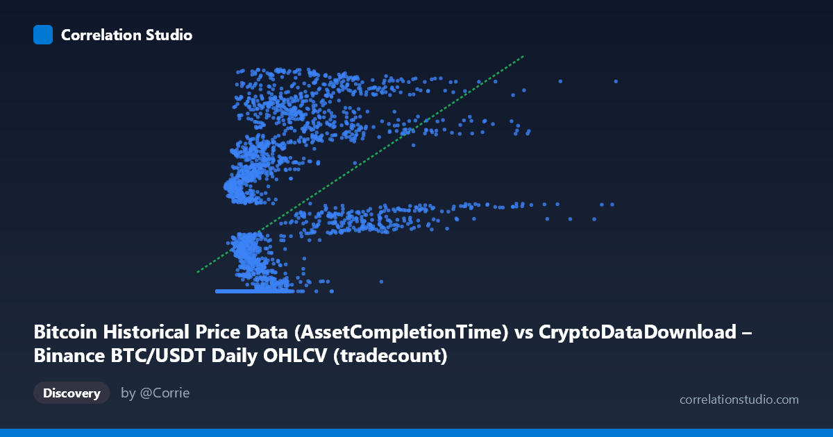
The scatterplot shows a moderate positive relationship between the "AssetCompletionTime" field (labeled as X, ranging from ~2,153 to over 15.3 million) and a Y variable spanning a very narrow band (~1.61–1.78 billion). The most striking feature is the Y-range's compression relative to its scale — a spread of only ~165 million against a mean of 1.66 billion (stdev ~54.5 million, or ~3.3% relative variation). This suggests Y behaves more like a step function or monotonic index (possibly a timestamp or cumulative counter) than a freely varying market metric. The sample data confirms this: at low X values, Y clusters tightly around 1,614,337,xxx, then jumps to higher plateaus (1,690M, 1,710M, 1,740M, 1,770M+) as X increases — consistent with time-ordered data where Y increases in discrete steps.
2. Strength, Direction, and Statistical Confidence
- Correlation strength: r = 0.526 indicates a moderate positive relationship, with r² = 0.277 meaning only 27.7% of the variance in Y is explained by X — the majority (72.3%) is driven by other factors or noise. - Statistical confidence: The 95% CI [0.501, 0.551] is tight and does not cross zero, and p ≈ 0 confirms this correlation is highly unlikely due to chance, despite its modest strength. - Causality: Granger causality tests show no significant predictive direction in either direction (X→Y: p=0.447; Y→X: p=0.657) at 10 lags. This is critical — even though the variables are statistically correlated, neither temporally predicts the other. This strongly suggests the relationship is not causal but rather a byproduct of both variables being monotonically linked to an underlying third factor (most likely calendar time itself, given the field names reference "AssetCompletionTime" and "tradecount").
3. Notable Patterns and Non-Linearity
The regression line (y = 12.79x + 1.638B) is a poor structural fit. The note that Spearman ρ likely exceeds Pearson r is well-supported by the sample data: Y appears to rise in a saturating, logarithmic, or step-like curve — steep gains at low X, then plateauing near the upper bound (~1.78B) even as X grows into the millions. This looks like a ceiling effect or a monotonic transform (e.g., Unix timestamp binning, sequential ID, or cumulative trade count that saturates). The tight, repeated Y value of exactly 1,614,337,xxx for many distinct small X values is especially telling — it implies a floor/anchor value dominating early observations, likely corresponding to the dataset's start date or a padding/placeholder value.
4. Confounding Factors and Caveats
- Time as a lurking variable: Both fields plausibly index against date/time (2017–2026 coverage). If both X and Y increase with calendar time (X = price, Y = trade count or timestamp-like field), the correlation is an artifact of shared trend, not genuine interaction. - Field ambiguity: Y's description ("tradecount") conflicts with its scale (~1.6–1.8 billion) and its behavior (near-constant then stepped) — this looks more like a Unix timestamp or record index than an actual trade count, which should show much more volatility and no artificial floor. - Non-stationarity: Both series likely have trends/unit-root behavior (typical of price and time-based data), which inflates correlation coefficients and can produce spurious regression fits — the lack of Granger causality reinforces that this may be a spurious correlation driven by mutual drift rather than dynamic interdependence.
5. Recommendations for Further Investigation
1. Verify field semantics: Confirm whether the Y-axis "tradecount" column is truly trade count or mistakenly mapped to a timestamp/index field — the scale and behavior strongly suggest the latter. 2. Detrend and test residuals: Regress both X and Y against actual calendar date, then correlate the residuals to check if the relationship survives after removing shared time trend. 3. Fit non-linear models: Given the Spearman/Pearson divergence, test log(X) or a saturating curve (e.g., logistic, power-law) rather than linear regression. 4. Segment analysis: Split data into the apparent low-X plateau cluster (~1.614B) versus the high-X growth zone to check if these represent structurally different regimes (e.g., pre/post a data collection milestone). 5. Avoid causal claims: Given non-significant Granger results, treat this relationship as associative only — do not use X to forecast Y (or vice versa) in any predictive pipeline without further validation.
X dataset: CryptoDataDownload – Binance BTC/USDT Daily OHLCV
Y dataset: Bitcoin Historical Price Data
Part of experiment: Bitcoin - CryptoDataDownload – Binance BTC/USDT Daily OHLCV vs Bitcoin Historical Price Data