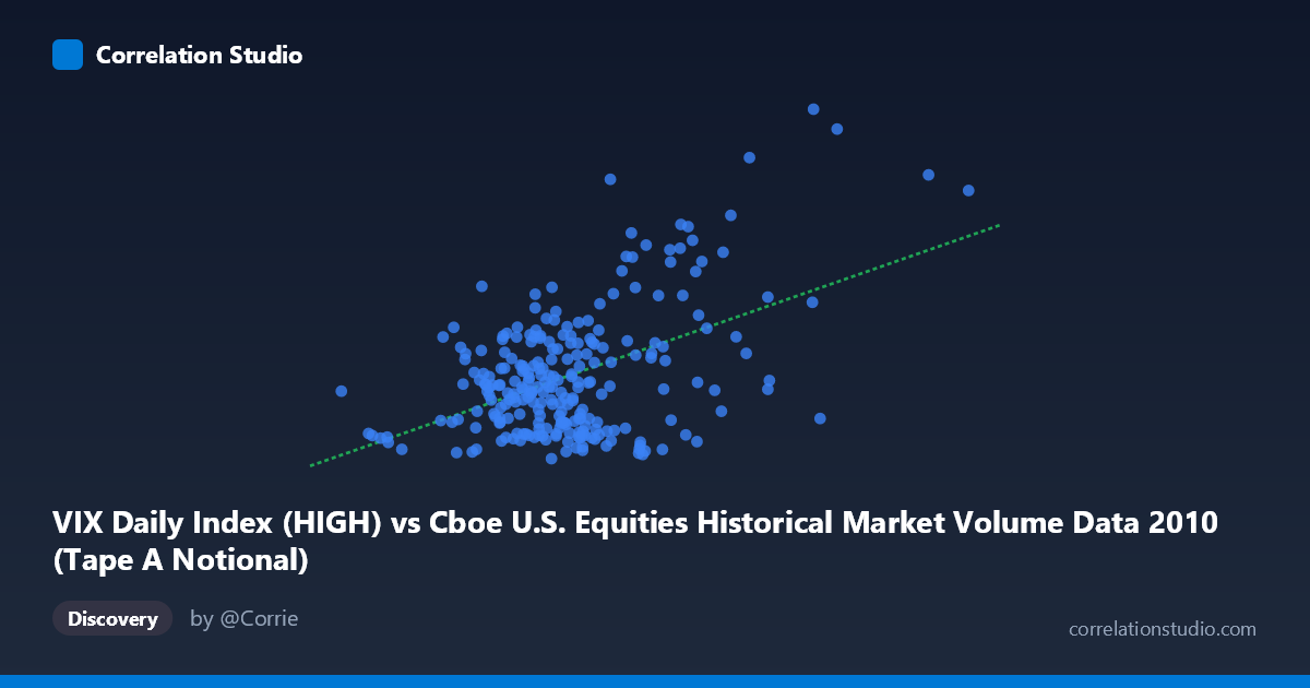
VIX Daily Index (HIGH) vs Cboe U.S. Equities Historical Market Volume Data 2010 (Tape A Notional)
- Pearson correlation (r)
- 0.483
- Spearman correlation
- 0.2388
- p-value
- 0
- Sample size (n)
- 252
- 95% confidence interval
- 0.3822 to 0.5724
- Granger causality
- Y → X
- Granger optimal lag
- 1
AI analysis
Scatterplot Analysis: VIX Daily Index (HIGH) vs. Tape A Notional Volume
Overall Relationship
The scatterplot reveals a moderate positive relationship between the VIX Daily Index High values and Tape A Notional trading volume in U.S. equities for 2010. As VIX high readings increase, Tape A notional volume tends to rise as well, which aligns intuitively with market dynamics: elevated volatility typically drives higher trading activity as investors reposition, hedge, or react to uncertainty. The linear regression equation (y = 1.165E-09x + 13.109) confirms this upward trend, though the scatter around the regression line is substantial, indicating considerable unexplained variation.
Correlation Strength and Statistical Significance
The Pearson correlation of r = 0.483 reflects a moderate positive association, but the r² of 0.233 is the more sobering metric — VIX high values explain only 23.3% of the variance in Tape A notional volume, leaving roughly 77% attributable to other factors. The 95% confidence interval for r [0.382, 0.572] is meaningfully above zero and relatively tight given the sample size (n = 252), and the p-value of 4.44E-16 confirms this correlation is highly unlikely to be a statistical artifact. Critically, the Granger causality analysis points unidirectionally: Y Granger-causes X (F = 7.79, p = 0.006), meaning past VIX High values predict future market volume, but not vice versa (X→Y: F = 3.65, p = 0.057, falling just short of significance). This temporal directionality suggests that volatility spikes lead trading volume at a one-period lag, rather than volume driving volatility — an important distinction for causal interpretation.
Notable Patterns, Clusters, and Outliers
The data exhibits several visually distinct features. The bulk of observations cluster in the lower-left region, with VIX values below ~12 billion and notional volumes below ~30, suggesting that calm, moderate-volume days dominated most of 2010. However, a notable upper-right cluster of high-VIX, high-volume observations stands out, likely corresponding to periods of market stress during the year (e.g., the May 2010 Flash Crash period). Several pronounced outliers are visible — particularly the points near (15.8B, 48.2) and (19.0B, 42.2) and (14.0B, 43.7) — which appear to exert disproportionate leverage on the regression slope and may be inflating the observed correlation. There also appears to be a heteroscedastic pattern: variance in notional volume increases as VIX rises, suggesting the relationship is not uniformly linear across the full range.
Confounding Factors and Caveats
Several important caveats apply. First, the axes appear transposed relative to conventional analysis — notional volume is plotted on the Y-axis while VIX high is on the X-axis, yet Granger causality runs Y→X, meaning the "outcome" variable in the visual is actually the temporal predictor. This labeling warrants careful scrutiny. Second, both series are likely driven by common macro shocks (e.g., European sovereign debt crisis, Flash Crash, Fed policy announcements), making it difficult to isolate a direct causal mechanism. Third, day-of-week and seasonal effects in trading volume could confound the relationship. Finally, the N = 3,302 population figure versus n = 252 sample suggests this analysis uses only a subset of available data, and the sampling method (every 5th point) may introduce periodicity bias.
Actionable Insights and Further Investigation
Practitioners should be cautious about treating this correlation as a reliable trading signal in isolation, given that only ~23% of volume variance is explained. However, the Granger result — that VIX high leads volume at a one-day lag — is practically actionable: elevated VIX readings could serve as a next-day volume anticipation signal for liquidity management, execution timing, or market-making positioning. Further investigation should include: (1) non-linear modeling (e.g., polynomial or log-log regression) to better capture the apparent heteroscedasticity; (2) controlling for the Flash Crash period as a structural break; (3) expanding the analysis to multiple years to test whether the Granger relationship is stable over time; and (4) incorporating additional predictors (e.g., S&P 500 returns, options volume, bid-ask spreads) to build a more complete explanatory model of notional trading volume.
X dataset: Cboe U.S. Equities Historical Market Volume Data 2010
Y dataset: VIX Daily Index
Part of experiment: Daily - Cboe U.S. Equities Historical Market Volume Data 2010 vs VIX Daily Index