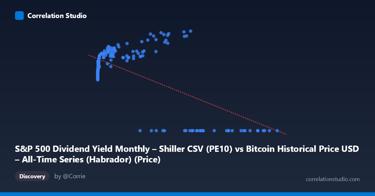
S&P 500 Dividend Yield Monthly – Shiller CSV (PE10) vs Bitcoin Historical Price USD – All-Time Series (Habrador) (Price)
- Pearson correlation (r)
- -0.638
- Spearman correlation
- 0.0682
- p-value
- 0
- Sample size (n)
- 189
- 95% confidence interval
- -0.7156 to -0.5449
- Granger causality
- Y → X
- Granger optimal lag
- 4
- Time coverage
- 2010-08-01 to 2026-04-01
- Recomputed on refreshed data
- 2026-10-13 (r was -0.638)
AI analysis
Analysis of X-Y Relationship
1. What the Visualization Reveals
The scatterplot shows a distinctly non-linear, bimodal relationship rather than a simple linear trend. For X values below roughly 60,000, Y clusters into a rising curve, climbing from ~20 at very low X to a peak near 35-38 as X approaches 40,000-60,000. However, once X exceeds approximately 60,000-65,000, Y drops sharply and flatlines at 0.00 for nearly every observation. This creates two visually distinct regimes: a "positive/curved" cluster at lower X values and a "zero-value" cluster at high X values, which is what drives the negative linear correlation despite the underlying relationship being far more complex than a straight line.
2. Strength, Direction, and Statistical Meaning
The reported r = -0.638 (r² = 0.407) indicates a moderate negative linear association, with about 41% of Y's variance explained by X — leaving the majority (59%) unexplained by this simple linear model. The 95% CI [-0.716, -0.545] is reasonably tight and excludes zero, and the p-value of 0 (effectively p < 0.001) confirms this correlation is highly unlikely to be due to chance given n=189. However, the linear r² substantially understates the true explanatory power here, since the actual pattern (rise-then-cliff-to-zero) is non-linear; a model capturing that structure would likely explain much more variance. On causality, the Granger test suggests Y→X (F=2.62, p=0.037) is significant while X→Y (F=2.33, p=0.058) just misses conventional significance — weak evidence that Y's past values help predict X better than the reverse, but both p-values are borderline, so this directional claim should be treated cautiously rather than as strong proof of causal precedence.
3. Notable Patterns and Outliers
The most striking feature is the hard zero-floor for Y at high X (roughly X 60,000), including points like (105620, 0.00), (97365, 0.00), (118670, 0.00) — these aren't scattered noise but a consistent structural break, suggesting a regime change, data-collection cutoff, or a variable that becomes structurally zero past a threshold (e.g., a rate/yield hitting a floor, or a metric undefined beyond a certain price level). In the lower-X regime, Y follows a smooth, monotonically increasing, concave curve (resembling a logarithmic or saturating growth curve) from Y≈20 at X near 0 up to Y≈38 near X=57,000. There's also a near-vertical cluster at very low X (X < 20) with Y ranging 20-23.5, indicating high sensitivity of Y to small changes in X at that end — classic log-scale behavior.
4. Confounding Factors and Caveats
Given the dataset labels, X and Y appear to represent Bitcoin price and an S&P 500/Shiller-derived metric (CAPE, dividend yield) mismatched across mismatched time series — the column descriptions are inconsistent/swapped, which raises serious concern about whether this pairing is meaningful or an artifact of merging two unrelated time series by date. The zero values are likely not "true zeros" but missing/unavailable data (e.g., Bitcoin price before genesis, or dividend yield data gaps) that got encoded as 0, which would badly distort both the correlation and Granger results. Time coverage (2010-2026) also spans vastly different Bitcoin market regimes (early adoption, multiple bull/bear cycles), and X's extreme right-skew (mean 20,533 vs stdev 29,894) means a few large values disproportionately influence the linear fit.
5. Actionable Insights
First, verify whether Y=0.00 values are genuine or represent missing/null data — if the latter, remove them and re-run the analysis, as this could substantially change both r and the causality direction. Second, apply a log transform to X (common for price/financial data spanning several orders of magnitude) before fitting, since the visible curve strongly resembles a log-linear or logistic relationship rather than a straight line — this would likely raise r² considerably. Third, given the borderline Granger p-values (0.037 vs 0.058), don't over-interpret directionality; test robustness with different lag structures and consider that both series may be driven by a common third factor (e.g., macro liquidity conditions, time trend) rather than one causing the other. Finally, double-check the column/dataset labeling, as the axis descriptions appear crossed or mislabeled, which should be resolved before drawing any domain conclusions about Bitcoin price vs. equity valuation metrics.
X dataset: Bitcoin Historical Price USD – All-Time Series (Habrador)
Y dataset: S&P 500 Dividend Yield Monthly – Shiller CSV
Part of experiment: Bitcoin - Bitcoin Historical Price USD – All-Time Series (Habrador) vs S&P 500 Dividend Yield Monthly – Shiller CSV