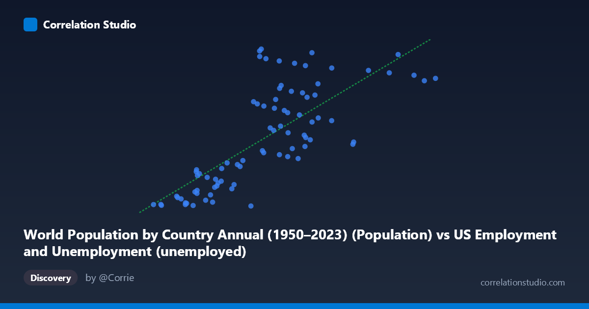
World Population by Country Annual (1950–2023) (Population) vs US Employment and Unemployment (unemployed)
- Pearson correlation (r)
- 0.752
- Spearman correlation
- 0.7816
- p-value
- 0
- Sample size (n)
- 83
- 95% confidence interval
- 0.6401 to 0.8326
- Granger causality
- None
- Granger optimal lag
- 10
- Time coverage
- 1941-01-01 to 2023-01-01
AI analysis
Scatterplot Analysis: World Population vs. US Unemployment
1. Overall Relationship
The scatterplot reveals a positive relationship between world population (x-axis) and US unemployment numbers (y-axis), with data spanning the period 1941–2023. As global population increases over time, US unemployment figures also tend to rise in absolute terms. The linear regression equation (y = 8827.04x + 42,840,300) captures this upward trend, though considerable scatter around the regression line is immediately apparent. Both variables are fundamentally time-indexed series that grow over the decades, which is a critical contextual factor in interpreting any apparent association.
2. Correlation Strength and Statistical Framing
The Pearson correlation of r = 0.752 indicates a moderately strong positive association, but the explanatory power is more sobering: R² = 0.5655 means only ~56.5% of the variance in US unemployment is accounted for by world population, leaving nearly 44% unexplained by this model alone. The 95% confidence interval for r [0.640, 0.833] is reasonably tight and excludes zero, and the p-value of 2.22×10⁻¹⁶ confirms the correlation is highly statistically significant — essentially ruling out chance as an explanation for the observed association. However, statistical significance here does not imply practical or causal meaning. Critically, Granger causality tests find no significant predictive directionality in either direction (X→Y: F = 0.655, p = 0.760; Y→X: F = 0.692, p = 0.727), even at an optimal lag of 10 periods. This means neither variable reliably predicts the other temporally, strongly suggesting the correlation reflects a shared underlying driver — time itself — rather than any genuine causal mechanism between population growth and US unemployment.
3. Notable Patterns, Clusters, and Outliers
Several features stand out within the scatter distribution. At lower population values (roughly 670–3,000 on the x-axis, corresponding to earlier decades), unemployment figures cluster tightly in the ~46–74 million range, suggesting relatively compressed variation in earlier years. At mid-to-high population values (~6,000–9,000), the data fans out considerably, with unemployment ranging from ~46 million to over 163 million — indicating dramatically increased variance at higher population levels, a possible sign of heteroscedasticity. Several apparent outliers deserve attention: points near (5,560; 46,410,179) and (5,996; 161,811,336) sit at similar x-values yet have dramatically different y-values, as do the cluster around x ≈ 6,000–6,100 where unemployment spans nearly the full y-range. This wide vertical spread in the middle of the x-distribution is inconsistent with a simple linear relationship and hints at non-linear or cyclical dynamics (e.g., recession years) overwhelming any population-driven trend.
4. Confounding Factors and Caveats
The most significant caveat is spurious correlation driven by shared temporal trend. Both world population and US absolute unemployment counts grow over time — population through demographic expansion, unemployment through labor force growth tied to a larger US population, not world population per se. This is a textbook case of two non-stationary time series producing an inflated correlation that evaporates under causal scrutiny (as the Granger tests confirm). Additional confounders include: business cycles and recessions (e.g., 2008–2009, COVID-2020) that cause unemployment spikes uncorrelated with world population; changes in BLS measurement methodology over 80+ years; and US-specific policy shifts (unemployment insurance coverage, labor force participation trends). The dataset pairing itself is conceptually unusual — world population is a global demographic aggregate while US unemployment is a country-specific labor market measure, making any direct causal narrative implausible on theoretical grounds alone.
5. Actionable Insights and Further Investigation
Given the spurious nature of this correlation, the most productive next steps would be: (1) Detrend both series (e.g., using first-differencing or percent-change transformations) before re-running correlation and Granger causality tests — a genuine relationship should survive detrending; (2) Substitute US population for world population as the x-variable, since US labor force size is the more theoretically relevant denominator; (3) Analyze the unemployment rate rather than absolute unemployed count, which controls for labor force growth and would eliminate much of the shared trend; (4) Investigate the high-variance cluster at mid-range x-values by flagging recession years to test whether cyclical effects explain the outliers; and (5) Apply cointegration tests (e.g., Engle-Granger) to formally assess whether any long-run equilibrium relationship exists beyond the common trend, before drawing any policy or analytical conclusions from this pairing.
X dataset: US Employment and Unemployment
Y dataset: World Population by Country Annual (1950–2023)
Part of experiment: Yearly - US Employment and Unemployment vs World Population by Country Annual (1950–2023)