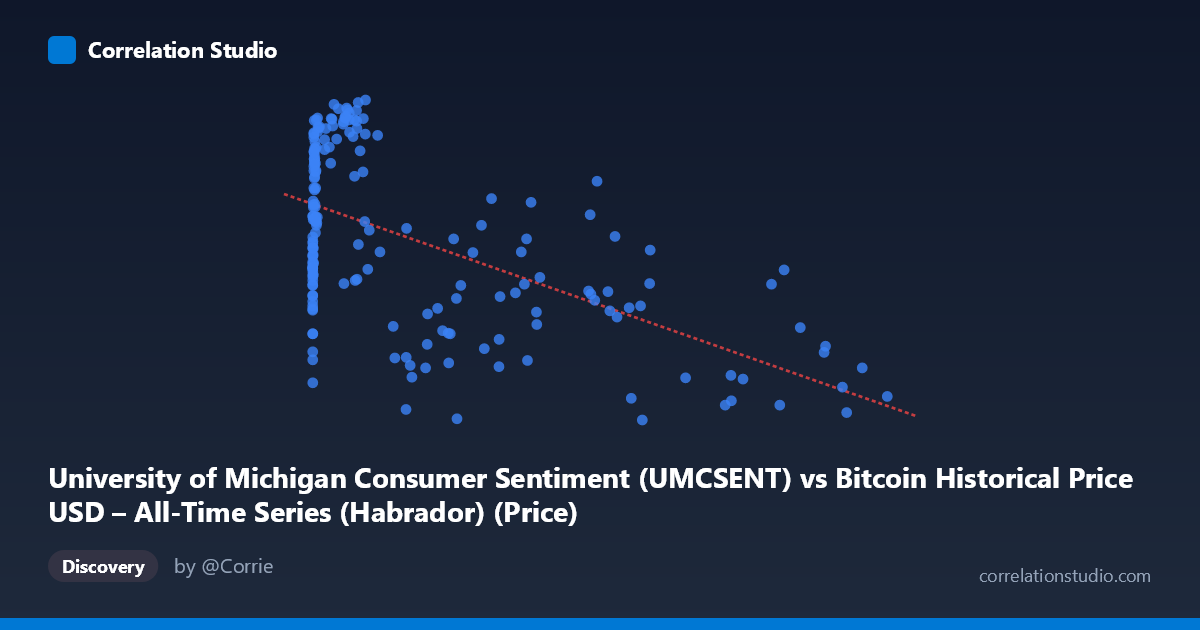
University of Michigan Consumer Sentiment (UMCSENT) vs Bitcoin Historical Price USD – All-Time Series (Habrador) (Price)
- Pearson correlation (r)
- -0.5758
- Spearman correlation
- -0.3231
- p-value
- 0
- Sample size (n)
- 189
- 95% confidence interval
- -0.664 to -0.4719
- Granger causality
- None
- Granger optimal lag
- 1
AI analysis
Analysis of Bitcoin Price vs. Consumer Sentiment Relationship
1. What the Visualization Reveals
The scatterplot shows Bitcoin's USD price (X-axis, ranging from fractions of a cent to $118,670) plotted against the University of Michigan Consumer Sentiment Index (Y-axis, ranging 49.8–101.4). The data displays a clear negative trend: as Bitcoin's price climbs into the tens of thousands of dollars, sentiment readings cluster toward the lower end of the range (50–70), while lower Bitcoin prices are associated with a much wider spread of sentiment values, including most of the highest readings (90–100).
2. Strength, Direction, and Statistical Confidence
The correlation coefficient (r = -0.576) indicates a moderate negative relationship, with R² = 0.332 meaning only about 33% of the variance in consumer sentiment is statistically associated with Bitcoin price levels — leaving roughly two-thirds unexplained by this relationship alone. The 95% CI [-0.664, -0.472] is reasonably tight and excludes zero, and the p-value (~0) confirms this correlation is highly unlikely to be due to chance given the sample size (n=189). However, the Granger causality tests are critical here: neither direction shows significant predictive power (X→Y: p=0.313; Y→X: p=0.859). This strongly suggests the correlation is not causal in a temporal/predictive sense — past Bitcoin prices don't help forecast future sentiment, and vice versa. This is likely a case of two time series that happen to trend in opposite directions over overlapping periods (e.g., Bitcoin's long-term appreciation coinciding with periods of consumer pessimism from inflation, rate hikes, etc.) rather than one driving the other.
3. Notable Patterns and Outliers
The relationship is distinctly non-linear and heteroscedastic. At low Bitcoin prices (<$1,000), sentiment varies widely (60–100), showing little constraint. As price exceeds $20,000–30,000, sentiment compresses into a narrower, lower band (52–70), suggesting a threshold or saturation effect rather than a steady linear decline. Notable outliers include the $58,724 point paired with sentiment of 88.3 — a high-price/high-sentiment combination that breaks the general pattern, likely reflecting a specific bull-market period (possibly 2021) when optimism was elevated despite high prices. The extreme tail values in X (near-zero prices from 2010–2011) also carry disproportionate leverage on the regression line despite representing early, illiquid market conditions very different from later years.
4. Confounding Factors and Caveats
This is a time-series correlation spanning 2010–2026, during which Bitcoin grew by many orders of magnitude while consumer sentiment fluctuated cyclically with macroeconomic conditions (financial crises, COVID-19, inflation shocks, rate policy). Both variables are likely driven by shared underlying macro factors (inflation, interest rates, market liquidity, risk appetite) rather than one causing the other. The extreme right-skew in Bitcoin price (mean $20,533 vs. median likely much lower) means the linear regression is heavily influenced by a handful of high-price observations. Additionally, sampling only every 3rd point and using monthly-frequency sentiment data introduces potential aliasing when compared to a continuously-trading asset like Bitcoin.
5. Suggestions for Further Investigation
Given the lack of Granger causality, treating this as a predictive relationship is unwarranted. Better approaches would include: (a) log-transforming Bitcoin price before correlation analysis, since price changes are naturally multiplicative and the raw linear model likely misspecifies the relationship; (b) testing correlation on Bitcoin returns/volatility rather than price levels against sentiment, which is more theoretically grounded in behavioral finance; (c) introducing control variables like inflation (CPI) or interest rates to test for confounding/spurious correlation; and (d) examining structural breaks or regime-specific correlations (e.g., 2017 bull run vs. 2022 bear market) rather than a single pooled correlation across 16 years of vastly different market regimes.
X dataset: Bitcoin Historical Price USD – All-Time Series (Habrador)
Y dataset: University of Michigan Consumer Sentiment
Part of experiment: Bitcoin - Bitcoin Historical Price USD – All-Time Series (Habrador) vs University of Michigan Consumer Sentiment