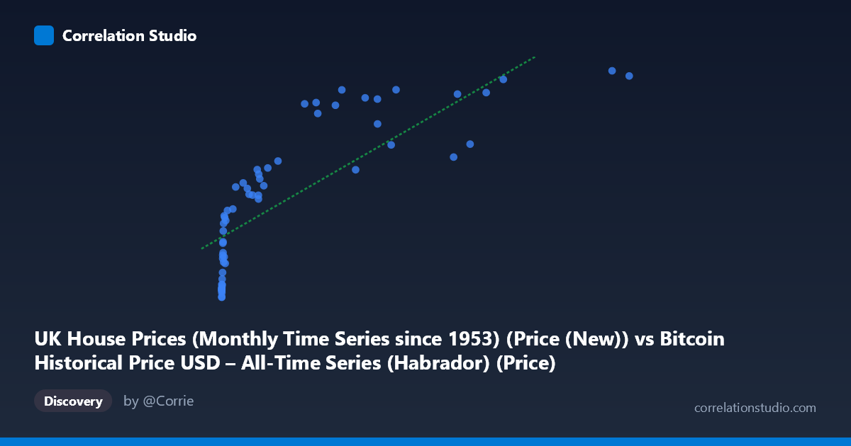
UK House Prices (Monthly Time Series since 1953) (Price (New)) vs Bitcoin Historical Price USD – All-Time Series (Habrador) (Price)
- Pearson correlation (r)
- 0.7992
- Spearman correlation
- 0.9682
- p-value
- 0
- Sample size (n)
- 60
- 95% confidence interval
- 0.6841 to 0.8754
- Granger causality
- None
- Granger optimal lag
- 10
- Time coverage
- 2010-08-01 to 2025-05-01
- Recomputed on refreshed data
- 2026-10-24 (r was 0.7992)
AI analysis
Analysis: Bitcoin Price vs. UK House Prices
1. Relationship Overview
The scatterplot displays a strong positive association between Bitcoin's historical USD price and UK house price index values, but the relationship is clearly non-linear. Data points cluster heavily at low X-values (Bitcoin under ~$10,000, which represents the vast majority of Bitcoin's history from 2010-2016), while a smaller number of high-X points (Bitcoin above $50,000, reflecting 2020-2025) pull the trend upward. The shape resembles a logarithmic or power curve rather than a straight line — Y rises steeply as X moves from near-zero to a few thousand, then the rate of increase moderates even as X climbs into the tens of thousands.
2. Strength, Direction, and Statistical Confidence
The Pearson correlation (r = 0.799, r² = 0.639) indicates a strong positive linear relationship, with the linear model explaining about 64% of the variance in Y. However, the note that Spearman ρ exceeds Pearson r confirms that a monotonic non-linear model (log or polynomial) would likely fit better than the linear regression equation shown (y = 1.499x + 206193). The 95% CI [0.684, 0.875] is reasonably tight given n=60, and the p-value (1.95E-14) confirms the correlation is highly unlikely to be due to chance. However, statistical significance of correlation does not imply causation — and this is reinforced by the Granger causality tests: neither direction (X→Y or Y→X) shows significant predictive power (p = 0.749 and p = 0.400 respectively). This strongly suggests both series are independently trending upward over time (both influenced by macro conditions, monetary expansion, time itself) rather than one driving the other.
3. Notable Patterns and Outliers
Several features stand out: - Dense low-X cluster: dozens of points with X < 1,000 span Y from ~167,000 to ~225,000, showing house prices varied considerably even while Bitcoin was negligible in value — this is the early-adoption noise period. - Compression/saturation at high X: points like (100700, 309918) and (96467, 313238) show Y plateauing near 300-313k even as X nearly doubles from ~58,000 to ~100,700, consistent with diminishing marginal association — a hallmark of a logarithmic relationship. - Mild non-monotonic wobble: some mid-range X points (e.g., 57302 → 257684; 61374 → 266030) sit below neighboring lower-X points (58254 → 298236), suggesting short-term Bitcoin volatility (crashes/corrections) doesn't track house price movements at all — supporting the "no Granger causality" finding.
4. Confounding Factors and Caveats
This is a classic case of spurious correlation via shared time trend. Both Bitcoin price and UK house prices have risen substantially over the 2010-2025 period due to entirely different but broadly correlated macro forces: quantitative easing, low interest rates (pre-2022), general asset price inflation, currency debasement (GBP and USD), and growing investor risk appetite. Neither market mechanically influences the other. Additionally, comparing a highly volatile speculative asset (Bitcoin) to a slow-moving, illiquid, regulated asset class (housing) on the same time axis conflates two very different price-formation processes. The small n (60 sampled points from a population of 290 monthly observations) and uneven X-distribution (heavily skewed toward low values) also limit how well the linear fit generalizes.
5. Actionable Insights
- Refit using a log-transformed X (log(Bitcoin price)) — this should substantially improve model fit given the Spearman/Pearson discrepancy and the visual saturation pattern. - Detrend both series (e.g., using year-over-year % changes or differencing) before testing correlation/causality — this isolates cyclical co-movement from shared secular trend and would likely reveal a much weaker or near-zero relationship. - Treat this correlation as coincidental/confounded by time, not usable for forecasting one asset from the other — the Granger results already confirm no predictive value in either direction. - Consider incorporating a common macro driver (e.g., M2 money supply, interest rates, or a global risk index) as a control variable to test whether it explains the shared upward trend better than either series explains the other.
X dataset: Bitcoin Historical Price USD – All-Time Series (Habrador)
Y dataset: UK House Prices (Monthly Time Series since 1953)
Part of experiment: Bitcoin - Bitcoin Historical Price USD – All-Time Series (Habrador) vs UK House Prices (Monthly Time Series since 1953)