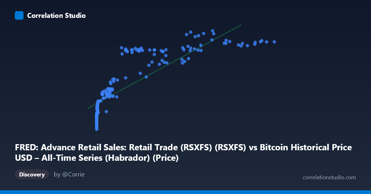
FRED: Advance Retail Sales: Retail Trade (RSXFS) (RSXFS) vs Bitcoin Historical Price USD – All-Time Series (Habrador) (Price)
- Pearson correlation (r)
- 0.8504
- Spearman correlation
- 0.9671
- p-value
- 0
- Sample size (n)
- 194
- 95% confidence interval
- 0.8061 to 0.8852
- Granger causality
- None
- Granger optimal lag
- 10
- Time coverage
- 2010-08-01 to 2026-09-01
- Recomputed on refreshed data
- 2026-10-24 (r was 0.8395)
AI analysis
Analysis: Bitcoin Price vs. Retail Sales (RSXFS)
1. What the Visualization Reveals
The scatterplot shows a strong positive association between Bitcoin's historical price and U.S. Advance Retail Sales, but the relationship is clearly non-linear. Data points trace a curve reminiscent of a logarithmic or power function: a dense cluster of low Bitcoin prices (under $1,000) maps to a wide range of retail sales values (~$330K–$440K), while Bitcoin prices climbing into the tens/hundreds of thousands correspond to retail sales compressing into a narrower upper band ($540K–$656K). This pattern is consistent with the note that Spearman's ρ exceeds Pearson's r — the rank-order relationship is tighter than the linear one, confirming the true relationship curves rather than following a straight line.
2. Strength, Direction, and Statistical Confidence
The Pearson correlation (r = 0.858) is strong and positive, with r² = 0.736 indicating that a linear model explains about 74% of the variance in retail sales using Bitcoin price as the predictor. The 95% CI [0.815, 0.891] is tight and excludes zero, and the p-value is effectively 0 — statistically, this is a highly reliable correlation given the sample. However, statistical significance here reflects shared trend/time dynamics, not causal mechanism or even necessarily a linear fit. Critically, Granger causality tests found no significant predictive direction in either direction (X→Y: p=0.80; Y→X: p=0.69). This means neither variable's past values help forecast the other's future values once autocorrelation is accounted for — the correlation is very likely driven by both series independently trending upward over the same calendar period, not by one influencing the other.
3. Notable Patterns and Outliers
Several features stand out: - Compression at scale: Points like (0.06, 313785) through (100, ~365000) show enormous relative changes in Bitcoin price with modest changes in retail sales — classic logarithmic-relationship signature. - Plateau at the high end: Once Bitcoin exceeds ~$60,000, retail sales values cluster tightly around $595K–$656K regardless of further price increases (e.g., $60K, $85K, $105K, $118K all yield similar Y values), suggesting the relationship flattens. - No visible reversals or negative excursions — the trend is monotonic, just not linear. - No extreme outliers deviate sharply from the curve; the scatter is well-behaved once log-transformed mentally.
4. Confounding Factors and Caveats
This is a textbook case of spurious correlation via shared time trend. Both Bitcoin price and U.S. retail sales have risen substantially from 2010–2026 due to entirely different underlying drivers: retail sales grow with population, inflation, and nominal GDP; Bitcoin price grew via adoption cycles, speculation, and halving events. The Granger non-causality result strongly supports treating this as trend confounding rather than a genuine economic relationship. Additionally, mismatched data frequencies (retail sales is monthly, Bitcoin is likely daily/higher-frequency, aggregated to n=189 paired points) and the enormous scale disparity in X (0.06 to 118,670) make the linear regression coefficient (slope ≈ 2.91) nearly uninterpretable in practical terms. Inflation is also unaddressed — nominal retail sales figures aren't adjusted for price-level changes over 16 years.
5. Recommendations
- Refit using a log or power-law model (e.g., log(X) vs. Y, or log-log) given the Spearman/Pearson divergence; this will likely raise explained variance and better represent the true functional form. - Detrend both series (e.g., first-differencing, or regressing out a time trend) before recomputing correlation — this tests whether any relationship survives after removing the shared upward drift. - Treat Granger results as decisive: do not use one series to forecast the other in trading or economic models; the lack of lead-lag structure is a strong red flag against causal interpretation. - Consider inflation-adjusting retail sales and comparing Bitcoin against a more theoretically linked variable (e.g., money supply M2, real interest rates) if the goal is to find genuine macro drivers of crypto prices.
X dataset: Bitcoin Historical Price USD – All-Time Series (Habrador)
Y dataset: FRED: Advance Retail Sales: Retail Trade (RSXFS)
Part of experiment: Bitcoin - Bitcoin Historical Price USD – All-Time Series (Habrador) vs FRED: Advance Retail Sales: Retail Trade (RSXFS)