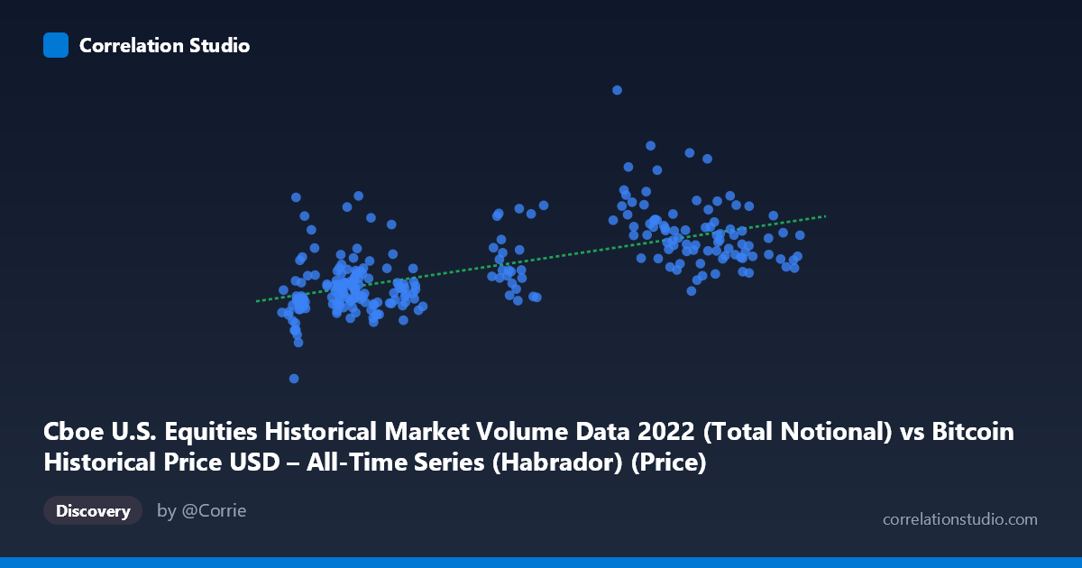
Cboe U.S. Equities Historical Market Volume Data 2022 (Total Notional) vs Bitcoin Historical Price USD – All-Time Series (Habrador) (Price)
- Pearson correlation (r)
- 0.6348
- Spearman correlation
- 0.6387
- p-value
- 0
- Sample size (n)
- 251
- 95% confidence interval
- 0.5546 to 0.7033
- Granger causality
- None
- Granger optimal lag
- 10
AI analysis
Analysis: Cboe Equities Volume vs. Bitcoin Price (2022)
1. What the Visualization Reveals
The scatterplot shows a moderate positive relationship between U.S. equities market volume (X) and Bitcoin price (Y) throughout 2022. As equities trading volume increases, Bitcoin price tends to rise as well, though the relationship is far from deterministic — there's substantial scatter around the regression line, particularly in the lower-X range (15,000–25,000) where Y values swing widely from ~21 billion to over 43 billion despite similar X values.
2. Strength, Direction, and Statistical Confidence
The correlation coefficient (r = 0.635) indicates a moderate-to-strong positive linear relationship, with r² = 0.403 meaning only about 40% of the variance in Bitcoin price is statistically associated with equities volume — leaving roughly 60% explained by other factors. The 95% confidence interval [0.555, 0.703] is reasonably tight given the sample size (n=251 of a 4,769-point population), and the p-value of ~0 confirms this correlation is highly unlikely to be due to chance. However, the Granger causality tests are the critical caveat here: neither direction (X→Y or Y→X) shows significant predictive power (p = 0.55 and p = 0.53 respectively). This means that despite the contemporaneous correlation, past values of equities volume do not help forecast future Bitcoin prices, and vice versa. The relationship appears to be a co-movement (likely driven by shared macro factors) rather than one variable temporally leading the other.
3. Notable Patterns and Outliers
Several structural features stand out: - Low-X cluster with high variance: Points with X between 16,000–23,000 show Y values ranging from ~21B to ~43B — this is the noisiest region of the dataset, suggesting volume alone poorly predicts price when volume is low. - Mid-range spikes: Values like (20,471, 43.3B) and (21,231, 39.2B) appear as outliers relative to neighboring points with similar X but much lower Y (~24-27B), indicating episodic decoupling. - Higher-X stabilization: In the 40,000+ range, Y values cluster more tightly between 31B–51B, suggesting the relationship may tighten (or saturate) at higher equity volumes, though a few high outliers exist (e.g., 40,716 → 51.2B). - No strong evidence of a non-linear (e.g., logarithmic or exponential) pattern — a linear fit seems like a reasonable first-order approximation, though the heteroscedasticity (variance changing across X) violates a strict linearity assumption.
4. Confounding Factors and Caveats
This correlation is very likely spurious or indirect rather than causal: - Both series may be jointly driven by macroeconomic conditions in 2022 (Fed rate hikes, inflation data, risk-off/risk-on sentiment) that simultaneously affected equities trading activity and crypto valuations. - 2022 was a uniquely volatile year (Fed tightening cycle, FTX collapse in November) — this correlation may not generalize to other periods with different market regimes. - The mismatched axis metadata (column labels appear swapped between "Habrador" and "Cboe" datasets) raises a data-integrity question that should be verified before drawing conclusions. - Daily volume and price are both non-stationary time series; correlating them directly (without differencing or detrending) risks the classic "spurious regression" problem common in financial time-series analysis.
5. Suggested Next Steps
- Test for cointegration rather than relying on raw correlation, given both series are likely trending/non-stationary. - Introduce a third variable (e.g., VIX, DXY, or Fed funds rate) to check if it explains the co-movement better than a direct link. - Segment by market regime (pre/post-FTX collapse, rate-hike announcement dates) to see if the correlation strength varies across sub-periods. - Given the null Granger causality result, do not use one series to forecast the other in a trading strategy; treat the relationship as descriptive/correlational only, not predictive. - Verify axis/column labeling to ensure the "X" and "Y" variables are correctly assigned to their described datasets.
X dataset: Bitcoin Historical Price USD – All-Time Series (Habrador)
Y dataset: Cboe U.S. Equities Historical Market Volume Data 2022
Part of experiment: Bitcoin - Bitcoin Historical Price USD – All-Time Series (Habrador) vs Cboe U.S. Equities Historical Market Volume Data 2022