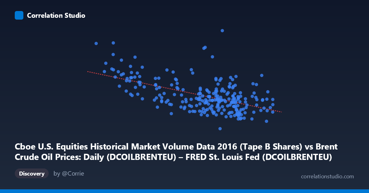
Cboe U.S. Equities Historical Market Volume Data 2016 (Tape B Shares) vs Brent Crude Oil Prices: Daily (DCOILBRENTEU) – FRED St. Louis Fed (DCOILBRENTEU)
- Pearson correlation (r)
- -0.5451
- Spearman correlation
- -0.4808
- p-value
- 0
- Sample size (n)
- 251
- 95% confidence interval
- -0.6266 to -0.4517
- Granger causality
- None
- Granger optimal lag
- 10
AI analysis
Analysis: Brent Crude Oil Price vs. Cboe Tape B Trading Volume (2016)
Relationship Overview The scatterplot reveals a moderate negative relationship between daily Brent crude oil prices (X-axis, USD/barrel) and Cboe Tape B equity share volume (Y-axis). As oil prices increase, trading volume in this equity segment tends to decline. The linear regression equation (y = -2,470,450x + 215,195,000) quantifies this inverse relationship, suggesting that for every $1 increase in Brent crude, Tape B volume decreases by approximately 2.47 million shares on average. This pattern is visually evident, particularly at the lower price range (roughly $26–$35/barrel) where several data points cluster at notably elevated volume levels, while the bulk of observations at higher prices ($40–$55) show comparatively compressed, lower volume figures.
Correlation Strength and Statistical Significance The Pearson correlation of r = -0.5451 indicates a moderate negative association, but the explanatory power is relatively limited: r² = 0.2971, meaning only about 29.7% of the variance in Tape B trading volume is explained by crude oil price levels. The remaining ~70% is driven by other factors entirely. The 95% confidence interval of [-0.6266, -0.4517] is reasonably tight and does not cross zero, and the p-value is effectively zero, confirming this correlation is statistically significant and unlikely to be a sampling artifact across the 251 paired observations drawn from a population of 3,622 trading days. However, statistical significance does not imply practical dominance — the majority of volume variation remains unexplained. Critically, Granger causality tests found no significant predictive direction in either direction (X→Y: F = 0.947, p = 0.491; Y→X: F = 0.706, p = 0.719), meaning oil prices do not temporally predict equity volume, nor does volume predict oil prices at the optimal 10-period lag. This strongly cautions against interpreting the correlation as a leading indicator relationship.
Notable Patterns, Clusters, and Outliers Several features stand out in the data. There is a distinct cluster of high-volume outliers at low oil prices — most visibly, the point at approximately (26.01, 209,001,199) and (27.59, 170,560,181), which correspond to the early-2016 period when Brent crude briefly collapsed to multi-year lows, triggering exceptional market activity. A secondary cluster of moderately elevated volume (120–145M shares) appears in the $30–$38 range. In contrast, the dense central mass of observations between $40–$55 shows relatively homogenous volume clustering around 80–110 million shares, with considerable scatter — suggesting that once oil prices normalized, the relationship weakened considerably. The point at (48.37, 138,827,428) is a notable upper outlier within the mid-price range, suggesting episodic volume spikes unrelated to oil price levels.
Confounding Factors and Caveats Several important caveats limit interpretation of this correlation. First, the relationship is almost certainly spurious or mediated by time: early 2016 was characterized simultaneously by a global oil price crash and heightened market volatility (VIX spikes), which would independently drive both low oil prices and high equity trading volume — the correlation may simply reflect shared sensitivity to a common macro volatility regime rather than any direct link. Second, Tape B specifically covers regional exchanges (NYSE Arca, NYSE American, etc.), whose volume dynamics are also driven by ETF activity, options expiration cycles, and index rebalancing events unrelated to crude oil. Third, the Granger causality failure confirms no reliable temporal lead-lag structure exists, undermining any mechanistic interpretation. Finally, with data confined to a single calendar year (2016), the observed pattern may reflect a one-time confluence of events rather than a durable structural relationship.
Actionable Insights and Further Investigation Given the moderate but incomplete correlation and absence of Granger causality, practitioners should avoid using oil price as a standalone predictor of Tape B volume. However, several follow-up analyses are warranted: (1) Introduce VIX or realized volatility as a control variable to test whether the oil-volume correlation disappears once market stress is accounted for — this would clarify whether the relationship is genuine or spurious; (2) Extend the time series beyond 2016 to assess whether this correlation is stable across different oil price regimes (e.g., 2020 crash, 2022 spike); (3) Disaggregate volume by sector — particularly energy-sector ETFs traded on Tape B venues — to test whether the relationship is concentrated in oil-sensitive instruments; and (4) Apply a non-linear or regime-switching model, since the scatterplot suggests the relationship may be threshold-dependent, with a much stronger effect at extreme low oil prices than in the normal operating range.
X dataset: Brent Crude Oil Prices: Daily (DCOILBRENTEU) – FRED St. Louis Fed
Y dataset: Cboe U.S. Equities Historical Market Volume Data 2016
Part of experiment: Daily - Brent Crude Oil Prices: Daily (DCOILBRENTEU) – FRED St. Louis Fed vs Cboe U.S. Equities Historical Market Volume Data 2016