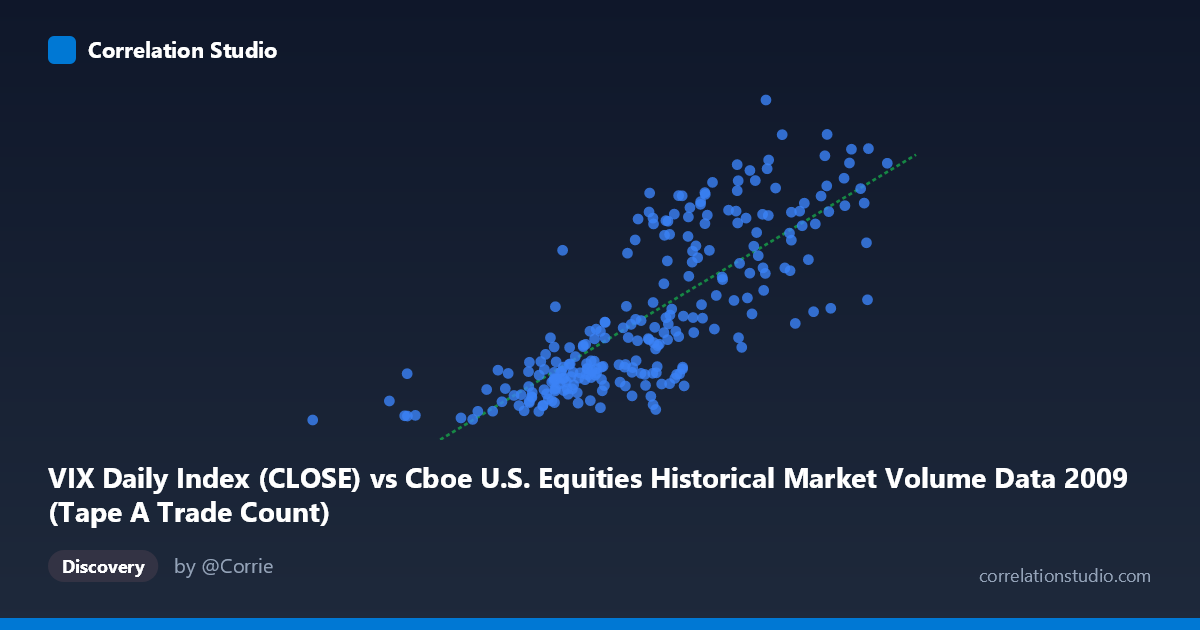
VIX Daily Index (CLOSE) vs Cboe U.S. Equities Historical Market Volume Data 2009 (Tape A Trade Count)

Pearson correlation (r): 0.7838
Spearman correlation: 0.8148
p-value: 0
Sample size (n): 252
95% confidence interval: 0.731 to 0.8272
Granger causality: None
Granger optimal lag: 1

AI analysis

Scatterplot Analysis: VIX Daily Index vs. Tape A Trade Count (2009)

Relationship Overview

The scatterplot reveals a moderately strong positive relationship between the VIX Daily Index (close) and Tape A Trade Count across U.S. equity exchanges in 2009. As VIX levels rise — indicating greater market fear and uncertainty — trading activity measured by Tape A trade counts also increases. This is intuitively consistent with market microstructure theory: elevated volatility drives higher transaction volumes as investors rebalance portfolios, execute hedges, and respond to rapidly shifting price signals. The linear regression equation (y = 1.83×10⁻⁵x + 1.693) confirms a positive slope, though the extremely small coefficient reflects the scale difference between the raw VIX values (X-axis spanning roughly 362K–2.55M in the dataset's native units) and trade counts on the Y-axis.

Correlation Strength and Statistical Significance

The Pearson correlation of r = 0.784 indicates a strong positive association, and the R² of 0.614 means that approximately 61.4% of the variance in Tape A trade counts is explained by VIX levels — a substantial but incomplete explanation. The 95% confidence interval of [0.731, 0.828] is relatively narrow given the sample of 252 paired observations drawn from a population of 3,232, lending high confidence that this is a genuine, robust relationship rather than a sampling artifact. The p-value of effectively zero reinforces this. However, the Granger causality results are notably absent of significance in either direction (X→Y: F=0.352, p=0.554; Y→X: F=0.186, p=0.667), meaning that despite a strong contemporaneous correlation, neither variable reliably predicts the other with a one-period temporal lag. This is an important distinction: the two variables move together, but there is no evidence of a leading/lagging predictive relationship at the daily frequency tested.

Patterns, Clusters, and Outliers

Several structural features are visible in the data. There appears to be a dense cluster at lower VIX and lower trade count values (roughly X < 1,500,000; Y < 30), representing calmer, more "normal" market days later in 2009 as the post-crisis environment stabilized. A second, more dispersed cluster occupies the upper-right region (high VIX, high trade counts), consistent with the acute volatility episodes of early 2009 during the financial crisis trough. The point at approximately (362,081; 19.47) stands out as a potential outlier representing an unusually quiet day, while observations near (2,320,189; 52.65) and (2,549,192; 49.30) anchor the high end. Some non-linearity may be present — the relationship appears to slightly fan or widen at higher VIX levels, hinting at possible heteroscedasticity where variance in trade counts grows with volatility.

Confounding Factors and Caveats

Several important caveats apply. First, 2009 is an exceptional year — spanning the depths of the Global Financial Crisis through an early recovery — meaning this correlation may be driven largely by a regime shift rather than a stable structural relationship. The dynamic might not generalize to other years with lower VIX ranges. Second, trade count inflation from algorithmic and high-frequency trading was accelerating in 2009, and mechanical HFT responses to volatility spikes could artificially amplify the correlation. Third, the axes appear to have a labeling inversion worth verifying: the dataset notes indicate VIX data is on the X-axis while Tape A Trade Count is on the Y-axis, but the source dataset labels are cross-referenced, suggesting the analyst should confirm column assignments before drawing firm conclusions. Finally, the remaining 38.6% unexplained variance points to other drivers — market news events, earnings seasons, Federal Reserve announcements, and liquidity conditions — that are not captured by VIX alone.

Actionable Insights and Further Investigation

Given the strong contemporaneous correlation but absent Granger causality, practitioners should treat VIX and trade volume as coincident indicators rather than using one to forecast the other at a daily lag. For trading infrastructure planning (e.g., capacity management), VIX level could serve as a same-day proxy for expected system load, but not as a next-day predictor. Further investigation should include: (1) testing longer lag structures (2–5 days) in Granger causality to see if predictive relationships emerge at different horizons; (2) segmenting by VIX regime (e.g., VIX < 25, 25–40, 40) to test whether the linear model holds across volatility environments; (3) adding controls for day-of-week effects, options expiration cycles, and macroeconomic announcements; and (4) extending the analysis across multiple years to determine whether this correlation is structurally stable or unique to the crisis environment of 2009.

X dataset: Cboe U.S. Equities Historical Market Volume Data 2009

Y dataset: VIX Daily Index

Part of experiment: Daily - Cboe U.S. Equities Historical Market Volume Data 2009 vs VIX Daily Index