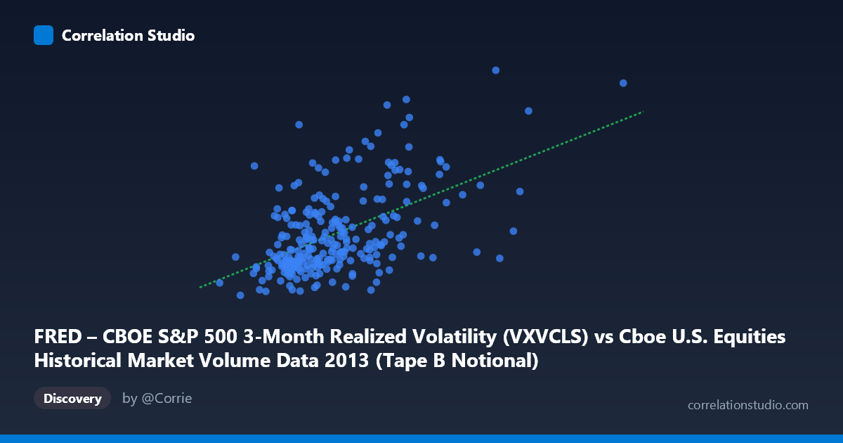
FRED – CBOE S&P 500 3-Month Realized Volatility (VXVCLS) vs Cboe U.S. Equities Historical Market Volume Data 2013 (Tape B Notional)
- Pearson correlation (r)
- 0.5318
- Spearman correlation
- 0.4798
- p-value
- 0
- Sample size (n)
- 252
- 95% confidence interval
- 0.437 to 0.615
- Granger causality
- None
- Granger optimal lag
- 1
AI analysis
Analysis: CBOE S&P 500 3-Month Realized Volatility vs. Tape B Notional Trading Volume (2013)
Relationship Overview
The scatterplot reveals a moderate positive relationship between CBOE S&P 500 3-month realized volatility (VXVCLS) and Tape B notional trading volume across 252 trading days in 2013. As realized volatility increases, Tape B notional volume tends to rise as well, consistent with the well-established finance literature connecting volatility regimes with elevated trading activity. The linear regression equation (y = 6.51×10⁻¹⁰x + 13.22) confirms this upward slope, though the relatively modest coefficient suggests the relationship, while real, is far from deterministic. The scatter around the regression line is visibly substantial, indicating that many days with similar volatility levels produce quite different notional volume outcomes.
Correlation Strength and Statistical Significance
The Pearson correlation of r = 0.532 indicates a moderate positive association, but the more practically informative statistic is r² = 0.283 — meaning realized volatility explains only 28.3% of the variance in Tape B notional volume. Nearly 72% of the variation in notional volume is driven by factors entirely outside this model. The 95% confidence interval for r [0.437, 0.615] is reasonably tight given the sample size of n = 252, and the p-value of essentially zero confirms this is not a chance finding in the sampled data. However, the Granger causality results tell a more nuanced story: neither direction of temporal predictive causality is statistically significant (X→Y: F = 1.17, p = 0.280; Y→X: F = 1.99, p = 0.160). This means that while the two variables move together contemporaneously, past values of volatility do not reliably predict future notional volume, and vice versa — a critical distinction for any trading or risk management application.
Notable Patterns, Clusters, and Outliers
The sample points reveal meaningful structural features worth noting. There is a dense cluster of observations in the volatility range of roughly 2.9–4.5 billion (X-axis) and Y values between approximately 14–16, suggesting a "normal regime" that dominated most of 2013. Several notable outliers are visible at the upper extremes: points such as (5,187,436,082, 19.84), (4,660,939,610, 18.82), and (4,425,354,898, 18.56) represent days with unusually high volatility and elevated notional volume simultaneously, potentially corresponding to specific macro events (e.g., the May 2013 "taper tantrum" or debt ceiling concerns). Conversely, a point near (2,577,414,404, 13.98) sits in a low-volatility, low-volume corner. There is also a hint of heteroscedasticity — the spread of Y values appears to fan out at higher X values — suggesting the relationship may be nonlinear or variance-amplifying at elevated volatility levels.
Confounding Factors and Caveats
Several important caveats temper interpretation. First, Tape B specifically covers NYSE American (AMEX) and regional exchange-listed securities, which may respond differently to broad market volatility than Tape A (NYSE) or Tape C (Nasdaq) listings — the correlation might not generalize across tapes. Second, 2013 was a structurally unusual year for U.S. equities: the Federal Reserve's taper discussions introduced episodic volatility spikes that don't represent typical market dynamics. Third, notional volume is price-sensitive — rising volatility often accompanies rising or falling prices, both of which inflate notional values independent of share volume changes, creating a potential mechanical coupling. Fourth, day-of-week effects, index rebalancing events, options expiration cycles, and ETF creation/redemption flows all independently drive Tape B notional volume and are uncontrolled here. The absence of Granger causality also warns against assuming any lead-lag economic mechanism.
Actionable Insights and Further Investigation
For practitioners, the moderate correlation suggests that realized volatility is a useful but insufficient predictor of Tape B notional volume — it could serve as one input in a multi-factor volume forecasting model, but should not be used in isolation. The lack of Granger causality at a 1-period lag suggests that intraday or same-day volatility measures may be more relevant than prior-day signals, warranting investigation at higher frequencies. Recommended next steps include: (1) testing nonlinear model specifications (e.g., log-log or polynomial regression) given the apparent heteroscedasticity; (2) segmenting the data by volatility regime (low/medium/high) to test whether the correlation strengthens in stress periods; (3) comparing this relationship across Tape A, B, and C to identify tape-specific dynamics; and (4) incorporating additional predictors such as VIX term structure slope, macro announcement calendars, and options expiration dates to improve the explained variance well beyond the current 28.3%.
X dataset: Cboe U.S. Equities Historical Market Volume Data 2013
Y dataset: FRED – CBOE S&P 500 3-Month Realized Volatility
Part of experiment: Daily - Cboe U.S. Equities Historical Market Volume Data 2013 vs FRED – CBOE S&P 500 3-Month Realized Volatility