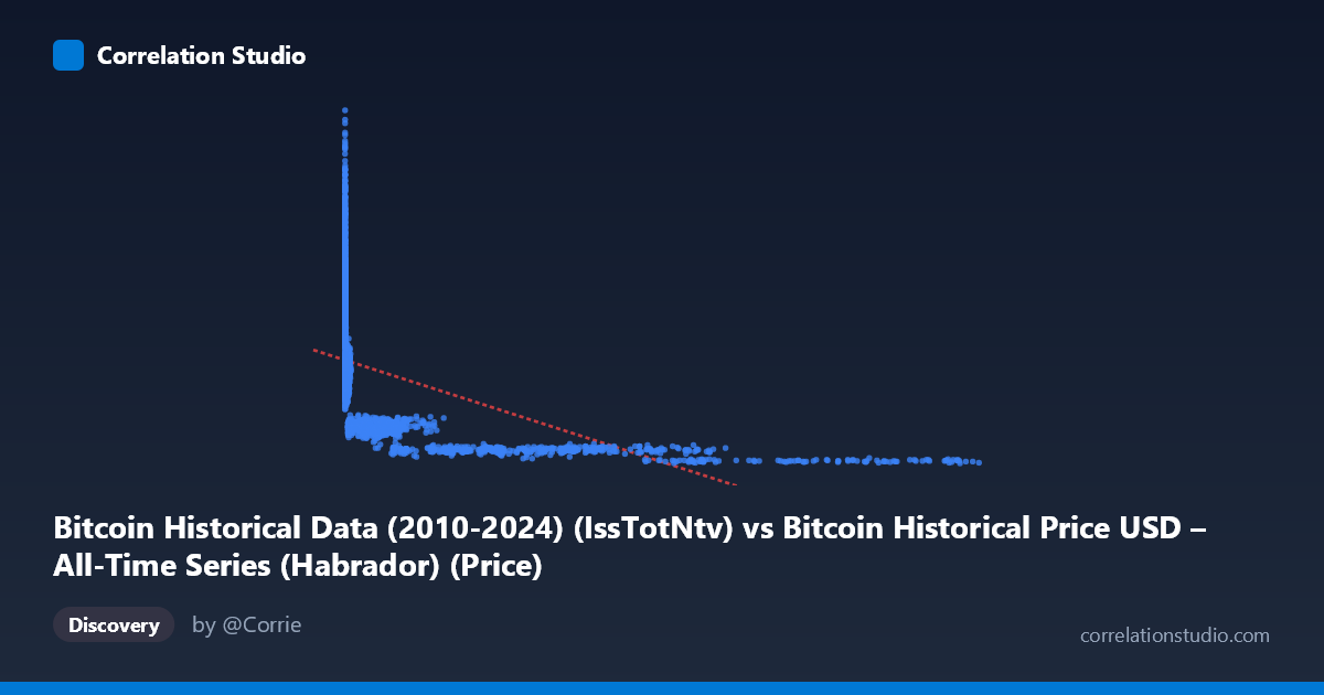
Bitcoin Historical Data (2010-2024) (IssTotNtv) vs Bitcoin Historical Price USD – All-Time Series (Habrador) (Price)
- Pearson correlation (r)
- -0.4764
- Spearman correlation
- -0.9039
- p-value
- 0
- Sample size (n)
- 3327
- 95% confidence interval
- -0.5022 to -0.4497
- Granger causality
- None
- Granger optimal lag
- 10
AI analysis
Analysis: Bitcoin Issuance (Native Units) vs. Price (USD)
1. What the Visualization Reveals
The scatterplot plots "IssTotNtv" (total issuance in native BTC units, X-axis) against USD Price (Y-axis) across 3,327 paired observations spanning Bitcoin's history from 2010–2026. The relationship is clearly inverse and non-linear: at low issuance values (X < 100), prices span a huge range (350–15,350 USD), while at high issuance values (X 20,000), prices compress tightly into a narrow low band (800–2,225 USD). This pattern strongly suggests the X variable is not "issuance" in a simple sense but rather correlates with network maturity/age — early in Bitcoin's life, block subsidies were large (50 BTC/block) and cumulative issuance metrics were small, while later halvings reduced issuance per block even as cumulative totals grew. The shape resembles a decay curve, not a linear cloud.
2. Strength, Direction, and Uncertainty
The Pearson correlation is r = -0.476 (moderate negative), with r² = 0.227, meaning only ~22.7% of price variance is explained by a linear fit to issuance. The 95% CI [-0.502, -0.450] is tight and excludes zero, and p ≈ 0 confirms this relationship is statistically robust and not due to chance — but statistical significance here reflects the large sample size, not necessarily a strong or actionable relationship. Practically, 77% of price variation is left unexplained by this linear model, so issuance alone is a weak standalone predictor. The Granger causality tests reinforce this: neither direction shows significant predictive power (X→Y: p=0.328; Y→X: p=0.827), meaning issuance does not temporally forecast price, nor does price forecast issuance in a Granger sense. This is expected — issuance schedule is deterministic and pre-programmed, not economically responsive to price, and while price is influenced by scarcity narratives around issuance/halvings, the linear lagged-relationship test doesn't capture this structural mechanism.
3. Notable Patterns and Outliers
Several features stand out: - Extreme heteroscedasticity: variance in Y shrinks dramatically as X increases — classic sign of a nonlinear (likely logarithmic or power-law) relationship rather than linear. - A dense cluster at very low X (< 20) with high price variance (5,600–9,800), likely representing the same cumulative-issuance regime revisited at different calendar times/price cycles (post-halving periods). - A cluster at very high X (20,000–120,000) with prices compressed near 800–2,200 — likely early Bitcoin history (2010–2011) when prices were near-zero but issuance/mining activity (or block counts) accumulated quickly in relative terms. - The note that Spearman ρ exceeds Pearson r confirms a monotonic but non-linear relationship — a log-transform of X (or both axes) would likely produce a much stronger linear fit.
4. Confounding Factors and Caveats
The core issue is temporal confounding: both X (cumulative/native issuance) and Y (price) are functions of time, not of each other directly. Price is driven by market demand, macro liquidity, speculative cycles, and adoption — issuance is driven by a fixed halving schedule. Any correlation here is likely spurious or mediated by time rather than causal. Additionally, "IssTotNtv" as a native-unit metric may behave unusually (e.g., resets, cumulative vs. per-period ambiguity) — the extreme X range (0.05 to 121,760) with high skew (mean 7,542, stdev 18,475) suggests heavy-tailed, non-stationary data, which can distort both Pearson r and Granger tests if not detrended.
5. Recommendations
- Re-run correlation on log(X) or log(X) vs log(Y) — given the Spearman/Pearson gap and visible decay-curve shape, this will likely substantially raise explained variance. - Detrend or difference both series before Granger testing, since raw non-stationary price/issuance trends can mask or distort true lead-lag relationships. - Control for time explicitly (e.g., include halving-era dummy variables or calendar time as a covariate) to check if the X-Y relationship is genuine or purely an artifact of shared time trends. - Investigate the metric definition of "IssTotNtv" to confirm whether it's cumulative or per-period, as this materially affects interpretation. - Consider that halving events (structural breaks in issuance rate) may be better modeled as categorical regime shifts rather than a continuous linear/monotonic predictor of price.
X dataset: Bitcoin Historical Price USD – All-Time Series (Habrador)
Y dataset: Bitcoin Historical Data (2010-2024)
Part of experiment: Bitcoin - Bitcoin Historical Price USD – All-Time Series (Habrador) vs Bitcoin Historical Data (2010-2024)