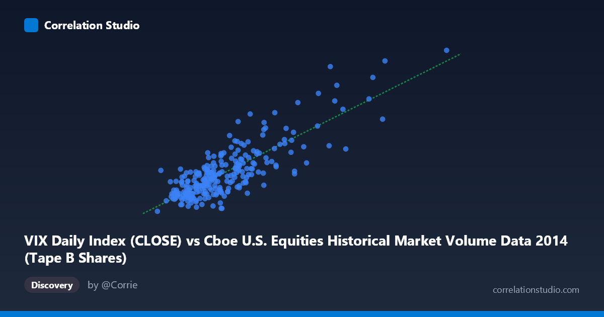
VIX Daily Index (CLOSE) vs Cboe U.S. Equities Historical Market Volume Data 2014 (Tape B Shares)

Pearson correlation (r): 0.8195
Spearman correlation: 0.728
p-value: 0
Sample size (n): 252
95% confidence interval: 0.7743 to 0.8563
Granger causality: None
Granger optimal lag: 1

AI analysis

Scatterplot Analysis: VIX Daily Index vs. Tape B Shares (2014)

Relationship Overview The scatterplot reveals a clear positive relationship between the VIX Daily Index (Close) and Cboe U.S. Equities Tape B Shares volume across 2014. As the VIX rises — reflecting heightened market uncertainty — Tape B share volume increases correspondingly. The linear regression equation (y = 9.11×10⁻⁸x + 7.32) captures this upward trend, and the data points broadly follow this trajectory, though with notable spread at higher VIX values. This is an intuitive finding: elevated fear and volatility typically drive increased trading activity as investors reposition, hedge, or liquidate holdings.

Correlation Strength and Statistical Robustness The correlation is strong and statistically meaningful (r = 0.8195, p ≈ 0), with the 95% confidence interval [0.7743, 0.8563] indicating a tight bound around the estimate — lending high confidence that the true relationship is robustly positive. Critically, r² = 0.6715 means that ~67% of the variance in Tape B share volume is explained by VIX levels, which is substantial for financial market data. However, ~33% of variance remains unexplained, signaling meaningful contributions from other factors. Despite this statistical strength, Granger causality tests reveal no significant temporal predictive direction in either direction (X→Y: F = 0.15, p = 0.70; Y→X: F = 0.04, p = 0.83), meaning that past VIX values do not reliably predict future Tape B volume — and vice versa — at the one-period lag tested. The correlation is therefore contemporaneous rather than predictive, a crucial practical distinction.

Patterns, Clusters, and Outliers The data exhibits a distinct two-regime structure. The majority of observations cluster tightly in the lower-left region (VIX roughly 38M–100M, Tape B roughly 11–17), suggesting relatively calm market conditions dominated 2014. However, a smaller but visible upper-right cluster (VIX closing values above ~140M–196M, Tape B ~20–26) represents elevated volatility periods — likely corresponding to market stress events such as the mid-October 2014 correction. Two particular points near (162M, 25.2) and (155M, 23.6) stand out as potential outliers that may disproportionately influence the regression slope. The spread around the regression line also widens at higher X values, suggesting heteroscedasticity — the relationship is less consistent during turbulent periods.

Confounding Factors and Caveats Several important caveats apply. First, the axes appear swapped in labeling (the dataset description places VIX on X but identifies Tape B Shares as originating from the VIX dataset file), which warrants verification before drawing conclusions. Second, common drivers — such as macroeconomic announcements, Federal Reserve communications, or geopolitical events — likely elevate both VIX and trading volume simultaneously, inflating the observed correlation without implying a direct mechanism. Third, the absence of Granger causality at lag-1 suggests the relationship may operate at intraday or multi-day lags not captured here. Finally, with N = 3,686 population observations but only n = 252 analyzed, sampling choices could affect representativeness.

Actionable Insights and Further Investigation Practitioners could use the contemporaneous VIX level as a same-day signal for expected Tape B volume, which has value for exchange capacity planning, liquidity provisioning, and execution strategy (e.g., expecting higher liquidity on high-VIX days). However, given the lack of Granger causality, VIX should not be used as a leading indicator for next-day volume decisions. Further investigation should: (1) test multiple lag structures (2–10 periods) for Granger causality to detect slower feedback loops; (2) apply breakpoint or regime-switching models to formally separate calm versus stressed market periods; (3) introduce control variables such as S&P 500 returns, bid-ask spreads, or macroeconomic release calendars to decompose the unexplained 33% variance; and (4) replicate the analysis across multiple years to assess whether the 2014 relationship is structurally stable or period-specific.

X dataset: Cboe U.S. Equities Historical Market Volume Data 2014

Y dataset: VIX Daily Index

Part of experiment: Daily - Cboe U.S. Equities Historical Market Volume Data 2014 vs VIX Daily Index