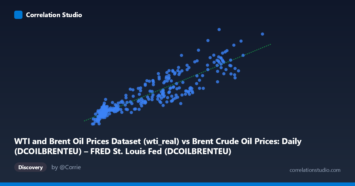
WTI and Brent Oil Prices Dataset (wti_real) vs Brent Crude Oil Prices: Daily (DCOILBRENTEU) – FRED St. Louis Fed (DCOILBRENTEU)
- Pearson correlation (r)
- 0.9032
- Spearman correlation
- 0.9219
- p-value
- 0
- Sample size (n)
- 295
- 95% confidence interval
- 0.8797 to 0.9222
- Granger causality
- None
- Granger optimal lag
- 4
AI analysis
Analysis: WTI Real vs. Brent Nominal Crude Oil Prices
1. Overall Relationship The scatterplot reveals a strong, positive, and broadly linear relationship between real (CPI-adjusted) WTI crude oil prices and nominal Brent crude oil prices spanning nearly four decades (1987–2026). As WTI real prices rise, Brent nominal prices rise in near-lockstep, which is expected given that these two benchmarks are the world's two dominant crude oil pricing references and are structurally linked through arbitrage, shared demand drivers, and global market integration. The regression line (y = 0.974x + 26.64) suggests that Brent nominal prices track WTI real prices at close to a 1:1 slope, with a meaningful positive intercept (~$26.64), likely reflecting the nominal inflation premium embedded in Brent's unadjusted prices relative to WTI's inflation-corrected series.
2. Correlation Strength and Statistical Significance The Pearson correlation of r = 0.903 is exceptionally strong, and the R² of 0.816 means that approximately 81.6% of the variance in Brent nominal prices is explained by WTI real prices — a remarkably high figure for two distinct financial time series measured on different bases. The 95% confidence interval of [0.880, 0.922] is narrow, confirming high precision in this estimate, and the p-value of ~0 eliminates any possibility this correlation arose by chance across the n = 295 paired observations. Practically, this confirms that the two benchmarks are deeply co-integrated in price discovery. However, the Granger causality results are notably absent of significance in either direction (X→Y: F = 1.32, p = 0.262; Y→X: F = 1.14, p = 0.340), meaning that at the optimal 4-period lag, neither series reliably predicts the other temporally beyond what each already contains. This is consistent with near-simultaneous price discovery in globally integrated oil markets rather than one benchmark leading the other.
3. Patterns, Clusters, and Outliers The scatterplot displays a clear dense cluster in the lower-left region (roughly WTI real $10–40 / Brent nominal $25–65), corresponding to the prolonged low-price environment of the late 1980s through early 2000s. A second, more dispersed cluster occupies the mid-to-upper range ($60–140 on both axes), reflecting the commodity super-cycle of 2003–2014 and the post-2021 recovery. Several points in the sample data show notable spread around the regression line — for example, (82.63, 131.60) and (90.36, 139.69) sit well above the fitted line, while (75.30, 73.28) and (62.90, 71.50) sit noticeably below it. These divergences likely correspond to periods of WTI-Brent spread widening, such as 2011–2013 when US pipeline bottlenecks at Cushing, Oklahoma caused WTI to trade at an unusual discount to Brent. The relationship also shows slight heteroscedasticity — variance around the regression line visibly increases at higher price levels, suggesting the two benchmarks decouple more during high-price, high-volatility regimes.
4. Confounding Factors and Caveats A critical interpretive caveat is the apples-to-oranges comparison at the heart of this analysis: WTI is measured in real (inflation-adjusted) terms while Brent is measured in nominal terms. This explains the positive intercept and means the correlation is partly driven by the secular inflation trend inflating Brent's nominal values over time. Any correlation analysis of this kind conflates genuine co-movement with a mechanical relationship introduced by deflation methodology. Additionally, temporal autocorrelation is a significant concern — daily oil prices are highly persistent, meaning effective degrees of freedom are far lower than the n = 295 sample suggests, and standard p-values likely overstate significance. Geopolitical shocks (Gulf Wars, OPEC supply cuts, COVID-19), currency fluctuations affecting USD-denominated prices, and structural market shifts (US shale revolution, ESG-driven demand changes) all represent confounders that can temporarily or permanently alter the WTI-Brent spread dynamics.
5. Actionable Insights and Further Investigation The near-unity slope (~0.97) and high R² suggest these series could serve as reasonable proxies for one another in most analytical contexts, but the residuals deserve targeted investigation — particularly those points deviating most from the regression line, which likely encode economically meaningful episodes of benchmark divergence. A recommended next step is to regress both series on a common nominal basis (or both real) to remove the inflation artifact and cleanly isolate spread dynamics. Analysts should also model the WTI-Brent spread as a standalone time series, testing for structural breaks around 2011 (shale boom) and 2020 (COVID demand collapse). Given the absence of Granger causality, vector error correction models (VECM) testing for cointegration would be more appropriate than predictive lag models. Finally, enriching the dataset with trading volume, inventory levels, and geopolitical risk indices could help explain the heteroscedastic high-price regime behavior and improve forecasting accuracy during volatile market conditions.
X dataset: Brent Crude Oil Prices: Daily (DCOILBRENTEU) – FRED St. Louis Fed
Y dataset: WTI and Brent Oil Prices Dataset
Part of experiment: Daily - Brent Crude Oil Prices: Daily (DCOILBRENTEU) – FRED St. Louis Fed vs WTI and Brent Oil Prices Dataset