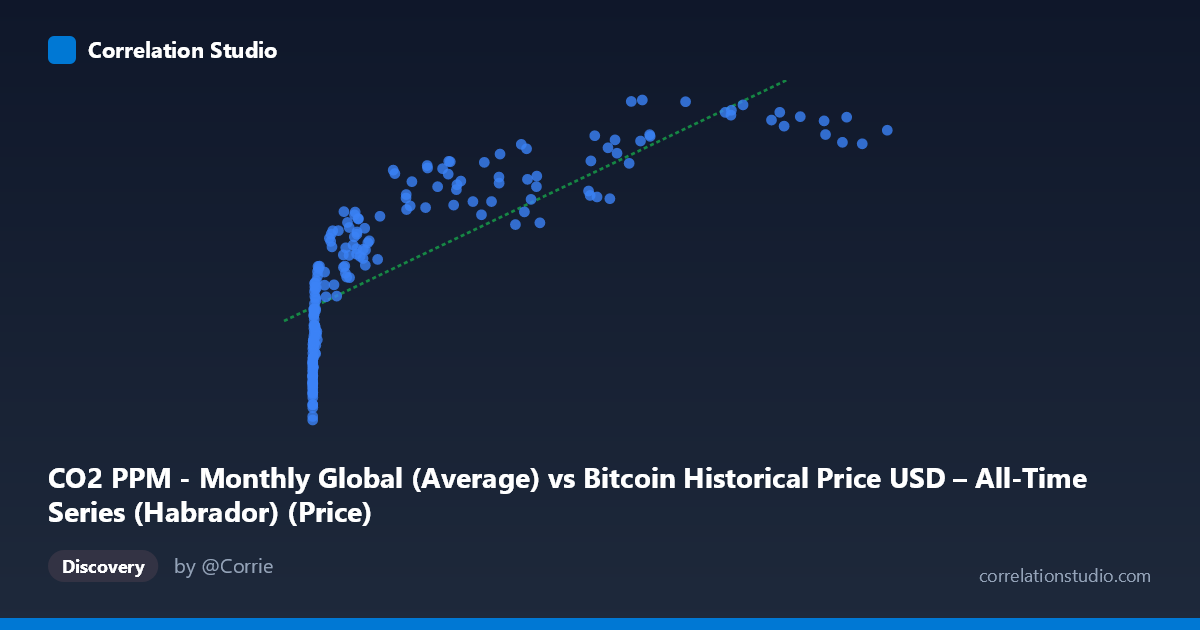
CO2 PPM - Monthly Global (Average) vs Bitcoin Historical Price USD – All-Time Series (Habrador) (Price)
- Pearson correlation (r)
- 0.8067
- Spearman correlation
- 0.9646
- p-value
- 0
- Sample size (n)
- 189
- 95% confidence interval
- 0.7503 to 0.8514
- Granger causality
- None
- Granger optimal lag
- 1
- Time coverage
- 2010-08-01 to 2026-04-01
- Recomputed on refreshed data
- 2026-10-20 (r was 0.8013)
AI analysis
Analysis: Bitcoin Price vs. Global CO2 PPM
1. What the Visualization Reveals
The scatterplot shows a strong positive association between Bitcoin's historical USD price and monthly global CO2 concentration (PPM). As Bitcoin's price climbs from fractions of a cent into the tens of thousands of dollars, CO2 readings rise in tandem from roughly 386 PPM to over 428 PPM. However, the relationship is visibly curved rather than linear: at low Bitcoin prices (under $1,000), CO2 values span a wide range (388–410 PPM) with steep sensitivity, while at high prices (above $50,000), the CO2 values compress into a narrower band (415–429 PPM). This pattern — rapid change at low X values flattening at high X values — is the classic signature of a logarithmic relationship, consistent with the note that Spearman's ρ exceeds Pearson's r.
2. Strength, Direction, and Statistical Meaning
The Pearson correlation (r = 0.80) indicates a strong positive linear association, with r² = 0.642 meaning the linear model explains about 64% of the variance in CO2 levels based on Bitcoin price — leaving over a third unexplained. The 95% CI [0.743, 0.847] is fairly tight and excludes zero, and the p-value of ~0 confirms this correlation is statistically robust and not due to chance. Critically, however, Granger causality tests show no significant predictive relationship in either direction (X→Y: p=0.73; Y→X: p=0.16). This means neither variable temporally leads or forecasts the other — the correlation is almost certainly driven by both series independently trending upward over the same calendar period, not by any causal or predictive linkage between Bitcoin markets and atmospheric chemistry.
3. Notable Patterns and Features
The data shows dense clustering at low X values (hundreds of points with X < 1,000, since Bitcoin traded near-zero for years) and sparse, spread-out points at high X values (Bitcoin's more recent multi-thousand-dollar era). The curvature is pronounced: CO2 rises quickly from ~386 to ~410 PPM while Bitcoin moves from $0 to ~$1,000, but then CO2 growth flattens significantly as Bitcoin surges past $50,000–$118,000. This is consistent with CO2's slow, steady, near-linear real-world annual increase (~2-3 PPM/year) mapped against Bitcoin's highly volatile, exponential-then-plateauing price trajectory — the "curve" is an artifact of time-alignment, not a functional relationship.
4. Confounding Factors and Caveats
This is a textbook example of a spurious correlation driven by a shared confounding variable: time. Both Bitcoin price and atmospheric CO2 have risen monotonically over the 2010–2026 window (CO2 due to continuous global emissions; Bitcoin due to adoption/speculation cycles), so any two upward-trending time series will show strong correlation regardless of any real connection. There is no plausible causal mechanism linking Bitcoin's price to global CO2 concentration at this level (aggregate global CO2 is driven by total fossil fuel combustion, land use, and seasonal biological cycles — Bitcoin mining's electricity draw is a rounding error against global emissions and wouldn't produce PPM-level atmospheric shifts on this timescale). The non-stationarity of both series (trending data) violates assumptions needed for correlation/regression to imply relationship, and is exactly why Granger causality — which accounts for temporal ordering — found nothing.
5. Actionable Insights
- Do not interpret this correlation as meaningful or actionable for trading, forecasting, or policy purposes; it is a time-trend artifact. - If a genuine relationship were of interest (e.g., Bitcoin mining's carbon footprint), better variables would be Bitcoin's energy consumption or hash rate correlated with regional/marginal emissions data, not global atmospheric PPM. - To properly test any relationship, de-trend both series (e.g., use year-over-year differences or growth rates rather than levels) and re-run correlation/Granger tests on the stationary residuals. - Given the visible curvature, if further modeling of X-Y is pursued for any reason, a log-transform of Bitcoin price (log(X)) should be tested against Y, which would likely raise the explained variance substantially over the naive linear fit.
X dataset: Bitcoin Historical Price USD – All-Time Series (Habrador)
Y dataset: CO2 PPM - Monthly Global
Part of experiment: Bitcoin - Bitcoin Historical Price USD – All-Time Series (Habrador) vs CO2 PPM - Monthly Global