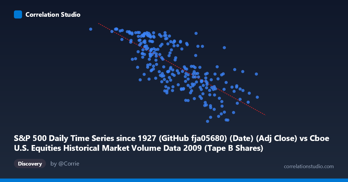
S&P 500 Daily Time Series since 1927 (GitHub fja05680) (Date) (Adj Close) vs Cboe U.S. Equities Historical Market Volume Data 2009 (Tape B Shares)

Pearson correlation (r): -0.7453
Spearman correlation: -0.7582
p-value: 0
Sample size (n): 252
95% confidence interval: -0.7956 to -0.6848
Granger causality: Bidirectional
Granger optimal lag: 10

AI analysis

Analysis: S&P 500 Adjusted Close vs. Cboe Tape B Shares (2009)

Relationship Overview The scatterplot reveals a moderately strong negative relationship between the S&P 500 adjusted closing price (X-axis) and Cboe Tape B share volume (Y-axis) across 2009 trading days. As the S&P 500 price level rises from its crisis lows (~33.8M range units) toward year-end recovery levels (~255.8M range units), Tape B share volume systematically declines. This inverse pattern is economically intuitive: during the market's distressed early-2009 period, panic-driven and forced selling generated exceptionally high trading volumes, while the subsequent recovery brought more orderly, lower-volume price appreciation. The linear regression equation (y = -2.01356E-06x + 1,243.72) confirms this descending trajectory.

Correlation Strength and Statistical Reliability The correlation of r = -0.7453 indicates a strong negative association, and the R² of 0.5555 means that approximately 55.5% of the variance in Tape B share volume is explained by the S&P 500 price level — a substantial but incomplete explanation, leaving roughly 44.5% attributable to other factors. The 95% confidence interval of [-0.7956, -0.6848] is relatively narrow and sits entirely in negative territory, providing high confidence that this inverse relationship is genuine and not a sampling artifact. The p-value of essentially zero, combined with a sample of 252 paired observations drawn from a population of 3,232, makes the finding statistically robust. The bidirectional Granger causality result (X→Y: F=2.45, p=0.0086; Y→X: F=2.79, p=0.0028) at a 10-period optimal lag is particularly notable — it suggests that not only does the S&P 500 price level temporally predict subsequent Tape B volume, but elevated Tape B volume also predicts future S&P price movements. This bidirectionality implies a feedback loop between market stress/activity and price discovery rather than a simple one-way driver.

Notable Patterns, Clusters, and Outliers Several structural features are visible in the sample points. There is a dense cluster of high-volume observations at lower price levels (roughly X < 120M, Y 1,000), corresponding to the January–March 2009 crisis period when the S&P 500 was near its generational lows and trading was frenetic. Conversely, observations at higher price levels (X 200M) tend to cluster with Tape B volumes below 900, reflecting the calmer H2 2009 recovery. A handful of outliers are notable: the point at approximately (33,822,027, 1,126) represents an extreme low-price/high-volume observation consistent with the very earliest 2009 trading days, while points like (254,504,132, 907) and (225,663,058, 929) show that even at high price levels, volume occasionally spikes — suggesting episodic news-driven activity. The relationship also appears to have mild non-linearity, with volume declining steeply at lower price levels and flattening somewhat as prices rise, hinting that a logarithmic or power-law fit might outperform the linear model.

Confounding Factors and Caveats Several important caveats temper interpretation. First, 2009 is a historically anomalous year — the market bottomed in March and then rallied ~65%, meaning the price-volume relationship is heavily influenced by a single extraordinary macro event (the Global Financial Crisis recovery) rather than representing a generalizable market structure. The strong correlation may largely be a spurious artifact of shared time-trend: both variables are driven by the crisis-to-recovery arc, making it difficult to disentangle genuine causal mechanisms from coincident temporal movement. Second, Tape B specifically covers NYSE American (AMEX) and regional exchange listings, which may have different liquidity profiles and investor bases than the broader S&P 500 universe, introducing a compositional mismatch. Third, regulatory changes (e.g., SEC circuit breaker rules implemented in 2009), algorithmic trading proliferation, and shifting market maker behavior could all independently affect Tape B volume. The Granger causality finding, while statistically significant, should not be interpreted as structural economic causation — it reflects predictive correlation at a 10-day lag within a single extraordinary year.

Actionable Insights and Further Investigation Practitioners should consider several follow-up analyses. Extending the time series across multiple years (pre-2008, 2010–present) would test whether this inverse price-volume relationship is persistent or unique to crisis regimes — a regime-switching model could formalize this distinction. The bidirectional Granger causality finding warrants deeper investigation: if Tape B volume genuinely leads S&P 500 price at 10-day lags, this could represent a exploitable signal for market participants monitoring regional exchange activity as a stress indicator. Decomposing volume into buyer- vs. seller-initiated trades (tick rule or quote rule classification) would clarify whether the high-volume/low-price period reflects panic selling or opportunistic buying. Additionally, controlling for the VIX or credit spreads as covariates would help isolate whether price is the true driver of volume or whether both are jointly determined by an underlying fear/uncertainty factor. Finally, testing whether a logarithmic or piecewise linear model improves on R² = 0.555 would quantify the non-linearity suggested by the data's visual structure.

X dataset: Cboe U.S. Equities Historical Market Volume Data 2009

Y dataset: S&P 500 Daily Time Series since 1927 (GitHub fja05680) (Date)

Part of experiment: Daily - Cboe U.S. Equities Historical Market Volume Data 2009 vs S&P 500 Daily Time Series since 1927 (GitHub fja05680) (Date)