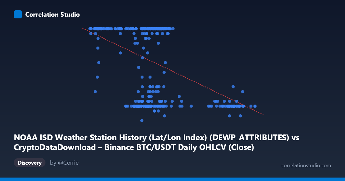
NOAA ISD Weather Station History (Lat/Lon Index) (DEWP_ATTRIBUTES) vs CryptoDataDownload – Binance BTC/USDT Daily OHLCV (Close)

Pearson correlation (r): -0.4701
Spearman correlation: -0.3044
p-value: 0
Sample size (n): 355
95% confidence interval: -0.5474 to -0.3848
Granger causality: None
Granger optimal lag: 1
Time coverage: 2024-01-01 to 2024-12-31

AI analysis

Scatterplot Analysis: DEWPATTRIBUTES vs. Close Price

1. Overview of the Relationship

The scatterplot displays a moderate negative correlation between the X variable (labeled as a weather attribute field but sourced oddly from BTC/USDT OHLCV data) and Y (labeled as "Close" but sourced from NOAA weather data). This mismatch in axis labeling versus data source is a critical caveat discussed below. Visually, the data shows a dense cluster of points in the X range of ~55,000–72,000 with Y values pinned heavily at the ceiling (24.00) and a secondary cluster of low Y values (7–12) in the same X range, alongside a sparser tail of points at higher X values (85,000–106,000) that consistently show low Y values (8–11).

2. Strength, Direction, and Statistical Confidence

The correlation coefficient (r = -0.4701, r² = 0.221) indicates a moderate negative linear relationship, but only 22.1% of the variance in Y is explained by X — meaning roughly 78% of Y's variability stems from other factors entirely. The 95% CI [-0.547, -0.385] is reasonably tight and excludes zero, and the p-value of ~0 confirms this correlation is statistically robust and not due to chance, given n=355. However, statistical significance should not be conflated with practical strength — this is a weak-to-moderate relationship, not a tight linear dependency. Critically, the Granger causality tests show no significant predictive direction in either direction (X→Y: p=0.58; Y→X: p=0.27), indicating that despite the contemporaneous correlation, neither series meaningfully forecasts the other at lag 1. This suggests the relationship, if genuine, is not a simple lead-lag dynamic.

3. Notable Patterns and Non-linearity

The most striking feature is bimodality in Y rather than a smooth linear trend: for X values between roughly 55,000–72,000, Y clusters sharply at either ~24 (ceiling, ~saturation) or single digits (~7–12), with few intermediate values. This bimodal clustering — rather than a diffuse cloud — suggests the linear regression (slope -0.000245) is capturing an average trend across what may actually be two distinct subpopulations or regimes, not a continuous linear decay. The high-X tail (85,000) is more consistently low (8–11), pulling the regression line downward and contributing disproportionately to the negative slope — these points may function as high-leverage observations.

4. Confounding Factors and Caveats

The dataset description contains a significant inconsistency: X is labeled as a NOAA weather attribute but its range/scale (39,568–106,133) and dataset origin point to BTC/USDT price data, while Y (range 5–24) is labeled "Close" price but its dataset source is NOAA weather station data. This suggests a column/label mismatch during data preparation — Y's tight bounded range (5–24) is far more consistent with a weather metric (e.g., wind speed, dew point in a transformed unit, or a coded attribute) than a crypto closing price, and vice versa for X. This mismatch must be resolved before drawing any domain conclusions. Additionally, spurious correlation is a real risk when pairing unrelated time series (crypto prices vs. weather) — shared temporal trends (e.g., seasonal patterns or dataset artifacts) can produce misleading r values absent any causal mechanism. The bimodal Y distribution also hints at a categorical or discretized variable rather than a purely continuous one, further undermining the linear model's appropriateness.

5. Recommendations

First, verify and correct the axis/column labeling — confirm which physical variable is actually on each axis before any substantive interpretation. Second, given the bimodal Y pattern, investigate whether a hidden categorical variable (e.g., season, station ID, or market regime) separates the two Y clusters — a mixture model or stratified analysis would likely outperform simple linear regression. Third, since Granger tests show no temporal predictability, treat this as a contemporaneous/structural association at most, not a forecasting relationship. Finally, consider non-linear or rank-based correlation (Spearman) and outlier-robust regression to test whether the high-X, low-Y tail is driving an otherwise weaker central-cluster relationship.

X dataset: CryptoDataDownload – Binance BTC/USDT Daily OHLCV

Y dataset: NOAA ISD Weather Station History (Lat/Lon Index)

Part of experiment: Bitcoin - CryptoDataDownload – Binance BTC/USDT Daily OHLCV vs NOAA ISD Weather Station History (Lat/Lon Index)