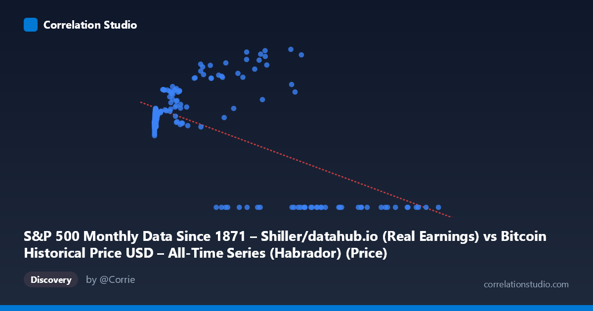
S&P 500 Monthly Data Since 1871 – Shiller/datahub.io (Real Earnings) vs Bitcoin Historical Price USD – All-Time Series (Habrador) (Price)

Pearson correlation (r): -0.6061
Spearman correlation: -0.1339
p-value: 0
Sample size (n): 194
95% confidence interval: -0.6882 to -0.5087
Granger causality: None
Granger optimal lag: 5
Time coverage: 2010-08-01 to 2026-09-01
Recomputed on refreshed data: 2026-10-24 (r was -0.5749)

AI analysis

Analysis: S&P 500 (Real Earnings) vs. Bitcoin Price

1. What the Visualization Reveals

The scatterplot shows a notably messy, non-linear relationship masquerading as a moderate negative linear correlation. Critically, the axis labels appear mismatched with the data description — the "X" values (ranging from 0.06 to 118,670) and their behavior strongly resemble Bitcoin price data (near-zero genesis values, exponential growth into the tens of thousands), while "Y" values clustering between 100-220 with many exact zeros resemble a bounded index or ratio (possibly Shiller Real Earnings or CAPE-like metric). This mismatch should be verified before drawing conclusions, as it affects interpretation of causality direction.

2. Strength, Direction, and Uncertainty

The correlation coefficient (r = -0.575, R² = 0.331) indicates a moderate negative relationship, but one that explains only 33% of variance — leaving two-thirds of Y's variation unexplained by X alone. The 95% CI [-0.663, -0.471] is reasonably tight and excludes zero, and the p-value of 0 confirms this correlation is statistically robust, not a artifact of sampling noise. However, statistical significance with n=189 (drawn from N=1,865) doesn't imply strong predictive power — R² of 0.33 means large residual variance remains.

The Granger causality result is intriguing: X→Y is significant (p=0.045) while Y→X is not (p=0.282), suggesting X's history has modest predictive value for Y at a 4-period lag — but F=2.49 is a weak effect, and Granger causality here reflects temporal precedence in the data, not necessarily true economic causation.

3. Notable Patterns and Outliers

The most striking feature is a cluster of exact zeros in Y across a wide range of X values (from ~27,000 to ~118,000) — this is almost certainly missing/null data coded as zero, not a genuine relationship, and it mechanically drives the negative correlation. Excluding these zeros, the real pattern among non-zero pairs shows Y generally rising with X (e.g., X=56,973→Y=217; X=44,354→Y=210; X=41,869→Y=190), which is the opposite sign of the reported overall correlation. There's also a dense cluster at low X (<1,000) with Y hovering around 110-135, suggesting a floor/baseline regime distinct from the high-X regime.

4. Confounding Factors and Caveats

- Zero-inflation artifact: The apparent negative correlation is likely an artifact of null-coded zeros at high X values, not a true inverse relationship. This should be treated as a missing-data problem, not a signal. - Non-stationarity: Both Bitcoin and equity/earnings series are non-stationary, trending series over a 2010-2026 window; naive correlation and Granger tests on non-stationary data risk spurious results unless differenced or detrended. - Axis/variable mismatch: The stated column names appear swapped, which could invalidate interpretation of "which variable causes which." - Extreme scale disparity: X spans 6 orders of magnitude (0.06 to 118,670), meaning linear correlation metrics are heavily influenced by a few large-X points.

5. Recommended Next Steps

1. Clean the zero values — determine if they represent missing data, and either impute or exclude them, then recompute correlation. 2. Log-transform X given its exponential-like distribution to stabilize variance and reveal the true functional form. 3. Verify variable assignment against source files to confirm which series is actually X vs. Y. 4. Use returns/differences rather than levels for both series to address non-stationarity before re-running correlation and Granger tests. 5. Treat the Granger result as suggestive only — replicate with proper stationarity testing (ADF) and consider it exploratory rather than confirmatory of economic causation.

X dataset: Bitcoin Historical Price USD – All-Time Series (Habrador)

Y dataset: S&P 500 Monthly Data Since 1871 – Shiller/datahub.io

Part of experiment: Bitcoin - Bitcoin Historical Price USD – All-Time Series (Habrador) vs S&P 500 Monthly Data Since 1871 – Shiller/datahub.io

Scatterplot: S&P 500 Monthly Data Since 1871 – Shiller/datahub.io (Real Earnings) vs Bitcoin Historical Price USD – All-Time Series (Habrador) (Price)