NOAA ISD Weather Station History (Lat/Lon Index) (WDSP_ATTRIBUTES) vs CryptoDataDownload – Binance BTC/USDT Daily OHLCV (Open)
- Pearson correlation (r)
- -0.4705
- Spearman correlation
- -0.3122
- p-value
- 0
- Sample size (n)
- 355
- 95% confidence interval
- -0.5478 to -0.3853
- Granger causality
- None
- Granger optimal lag
- 1
AI analysis
Analysis of X–Y Correlation
1. Overview of the Relationship
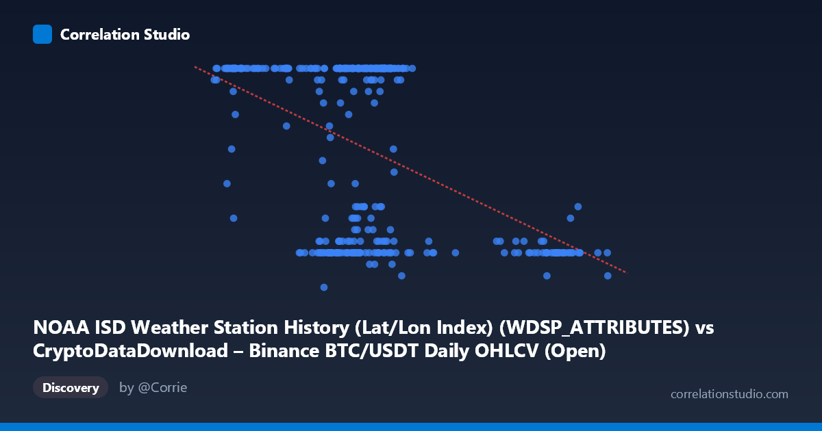
The scatterplot depicts a moderate negative linear relationship between the two variables, with a correlation coefficient of r = -0.4705. Visually, the data does not form a tight linear band but rather a dense, banded cluster: the majority of Y-values sit at either the low end (~7-12) or high end (~19-24), with relatively few points in the middle range. This bimodal clustering in Y, combined with a wide X range (~39,568 to ~106,134), suggests the relationship is driven more by distinct regimes or clusters of X than a smooth continuous decay.
2. Strength, Direction, and Statistical Confidence
The negative correlation (r = -0.47) indicates that as X increases, Y tends to decrease, but the r² of 0.2214 means only about 22% of the variance in Y is explained by X — the remaining ~78% is attributable to other factors, noise, or non-linear structure not captured by this simple linear model. The 95% confidence interval [-0.5478, -0.3853] is reasonably narrow and does not cross zero, and the p-value (effectively 0) confirms the correlation is statistically significant and unlikely due to chance, given n=355. However, statistical significance should not be conflated with practical predictive strength — an r² of 0.22 leaves substantial unexplained variability. Critically, the Granger causality tests show no significant predictive direction in either direction (X→Y: p=0.71; Y→X: p=0.26), meaning past values of one series do not meaningfully help forecast future values of the other. This strongly suggests the correlation is contemporaneous/structural rather than causal or lead-lagged in time.
3. Notable Patterns and Clusters
The data shows clear clustering behavior: a dense concentration of points around X = 60,000–70,000 with Y values sharply split between low (~8-12) and high (~21-24) bands, and a second cluster at higher X values (~90,000-100,000) almost exclusively associated with low Y values (~8-11). Very few points populate the middle X range (75,000-90,000) or middle Y range (13-18), producing a somewhat "gap" or bimodal appearance rather than a continuous cloud. This pattern hints at underlying regime-switching or threshold behavior — e.g., Y behaving like a near-binary/categorical variable conditioned loosely on X — rather than a smooth linear response.
4. Confounding Factors and Caveats
The variable labels appear mismatched or corrupted in the metadata (X is labeled as a NOAA weather station index while actually appearing to be BTC/USDT price data, and Y is labeled as BTC OHLCV Open while resembling a weather-station-like categorical/integer index in the 5-24 range). This strongly suggests a data-pipeline or column-mapping error, and any substantive interpretation (financial or meteorological) should be treated with caution until the source columns are verified. Additionally, with time-series data spanning a full year, autocorrelation within each series (common in both price data and seasonal weather data) can inflate apparent correlation strength independent of any real relationship — the Granger non-causality result reinforces that this may be a spurious or confounded association rather than a mechanistic one.
5. Recommendations for Further Investigation
First, verify and correct the axis/column labeling to ensure X and Y are drawn from their intended datasets — this is the most urgent step before drawing domain conclusions. Second, given the bimodal/clustered appearance of Y, consider treating Y as a categorical or discretized variable and applying clustering analysis, logistic regression, or a mixture model rather than continuous linear regression, since a linear r²=0.22 likely understates the true structure. Third, explore whether an omitted third variable (e.g., time, season, or an external market/weather driver) jointly influences both series, producing a non-causal correlation. Finally, since Granger tests show no lead-lag predictability, any forecasting application should not rely on one series to predict the other's future values; instead, focus on contemporaneous relationships or search for a shared external driver.
X dataset: CryptoDataDownload – Binance BTC/USDT Daily OHLCV
Y dataset: NOAA ISD Weather Station History (Lat/Lon Index)
Part of experiment: Bitcoin - CryptoDataDownload – Binance BTC/USDT Daily OHLCV vs NOAA ISD Weather Station History (Lat/Lon Index)