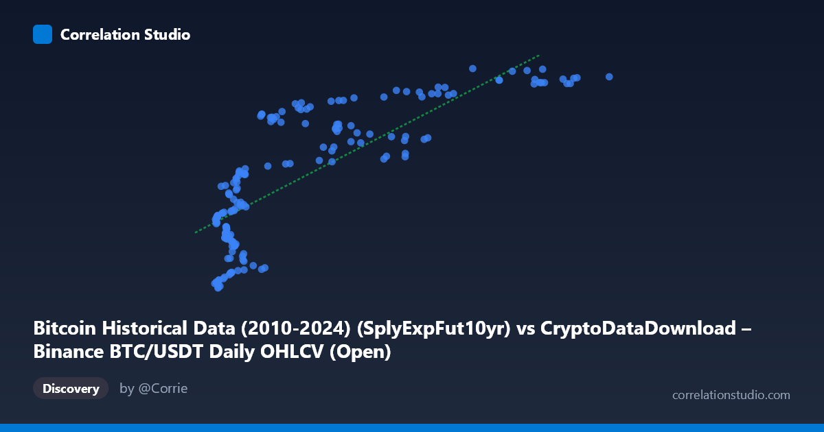
Bitcoin Historical Data (2010-2024) (SplyExpFut10yr) vs CryptoDataDownload – Binance BTC/USDT Daily OHLCV (Open)
- Pearson correlation (r)
- 0.8018
- Spearman correlation
- 0.8301
- p-value
- 0
- Sample size (n)
- 180
- 95% confidence interval
- 0.7426 to 0.8486
- Granger causality
- None
- Granger optimal lag
- 10
- Time coverage
- 2017-08-20 to 2026-02-02
AI analysis
Analysis: SplyExpFut10yr vs. BTC/USDT Open Price
1. Relationship Overview
The scatterplot depicts a positive, non-linear relationship between an on-chain supply metric ("SplyExpFut10yr" — a Bitcoin supply projection) and the daily BTC/USDT open price. The data shows a clear upward trend, but the shape is distinctly curved rather than a straight line: Y values climb rapidly in the low-X range (X < 20,000), then flatten into a plateau as X increases beyond ~60,000, with Y asymptotically approaching ~20,780,000–20,828,000. This logarithmic/saturating curve pattern suggests the linear model, while statistically significant, is not the ideal functional form for this data.
2. Strength, Direction, and Uncertainty
The Pearson correlation (r = 0.80) indicates a strong positive linear association, with r² = 0.643 meaning the linear model explains about 64% of the variance in Y — a substantial but incomplete share, leaving over a third of variance attributable to other factors or non-linear structure. The 95% confidence interval [0.743, 0.849] is reasonably tight given n=180, and the p-value of ~0 confirms this correlation is highly unlikely to be due to chance. However, statistical significance here reflects strength of linear association, not causation. Critically, the Granger causality tests show no significant predictive direction in either direction (X→Y: p=0.451; Y→X: p=0.673) at the optimal lag of 10 periods. This means neither series reliably helps forecast future values of the other over time — the strong contemporaneous correlation is not matched by temporal lead-lag structure, undermining any causal or predictive interpretation.
3. Notable Patterns and Outliers
The most salient feature is the saturation/plateau pattern at high X values — once X exceeds ~70,000–100,000, Y compresses into a narrow band (~20,750,000–20,828,000), indicating diminishing marginal sensitivity of price to this supply metric at scale. Conversely, in the low-X region (X < 10,000), Y varies substantially (20,209,550 to over 20,540,000), showing higher volatility/sensitivity. There's also a visible cluster around X≈4,000–12,000 with wide Y-scatter, suggesting this region contains noisier or more heterogeneous observations — possibly corresponding to a different market regime or time period. No extreme outliers break the overall curve shape, but the point (76968.22, 20828425.00) marks the Y maximum, sitting slightly above the general plateau trend.
4. Confounding Factors and Caveats
Both variables are derived from the same underlying BTC/USDT price series (X is a supply-side projection metric, Y is literally the OHLCV Open price from the same exchange), so this is very likely a mechanical/definitional relationship rather than two independent phenomena correlating. "SplyExpFut10yr" (Supply Expected in Future 10yr) is likely a function of Bitcoin's known halving-based issuance schedule, which is monotonically related to time — and price also trended upward over the 2017–2026 window. This creates a classic spurious correlation via shared time trend: both series moved together because they're both functions of calendar time/market cycles, not because one drives the other. The non-stationarity of price data (trending, autocorrelated) also violates assumptions needed for meaningful correlation/Granger inference without differencing.
5. Suggestions for Further Investigation
Given the mechanical relationship and lack of Granger causality, this correlation should not be used for predictive trading or causal claims. Recommended next steps: (1) fit a non-linear model (log or power function) given the visible saturation curve, which should substantially improve fit over the linear R²=0.643; (2) difference or detrend both series (e.g., % change, log-returns) before re-testing correlation and Granger causality to control for the shared time trend; (3) clarify what "SplyExpFut10yr" actually represents — if it's a deterministic supply schedule, correlating it with price is more a study of adoption/scarcity narrative timing than a genuine bivariate relationship; (4) segment the analysis by time period (e.g., pre/post 2021 bull cycle) to check if the relationship is stable or driven by a specific market regime.
X dataset: CryptoDataDownload – Binance BTC/USDT Daily OHLCV
Y dataset: Bitcoin Historical Data (2010-2024)
Part of experiment: Bitcoin - CryptoDataDownload – Binance BTC/USDT Daily OHLCV vs Bitcoin Historical Data (2010-2024)