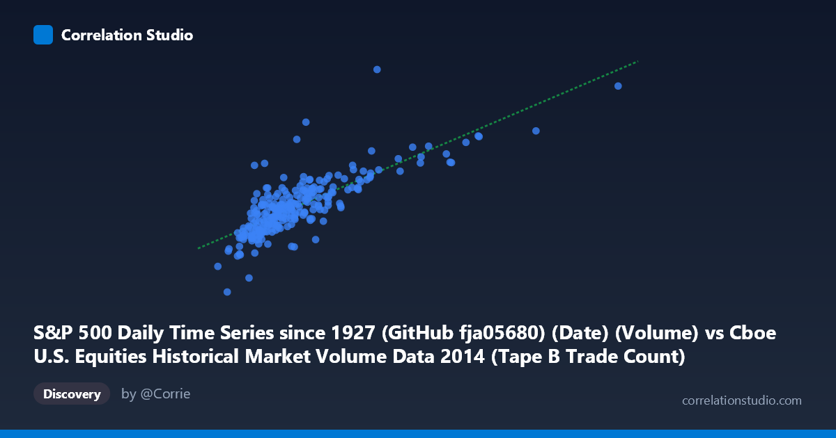
S&P 500 Daily Time Series since 1927 (GitHub fja05680) (Date) (Volume) vs Cboe U.S. Equities Historical Market Volume Data 2014 (Tape B Trade Count)
- Pearson correlation (r)
- 0.7901
- Spearman correlation
- 0.7729
- p-value
- 0
- Sample size (n)
- 252
- 95% confidence interval
- 0.7387 to 0.8324
- Granger causality
- None
- Granger optimal lag
- 10
- Time coverage
- 2014-01-02 to 2014-12-31
AI analysis
Scatterplot Analysis: S&P 500 Daily Volume vs. Cboe Tape B Trade Count (2014)
Relationship Overview The scatterplot reveals a clear positive linear relationship between the S&P 500 daily trading volume and the Cboe U.S. Equities Tape B trade count across the 2014 trading year. As daily volume on the S&P 500 increases, the number of Tape B trades rises correspondingly, which is intuitive — both metrics are expressions of overall market activity. The linear regression equation (y = 6,833.99x + 1.841×10⁹) captures this upward trend well, and the scatter of points broadly follows the fitted line across the volume range of roughly 110,000 to 676,000 units. The relationship reflects a common underlying driver: days with elevated investor participation tend to generate higher transaction counts across multiple market venues simultaneously.
Correlation Strength and Statistical Significance The correlation coefficient of r = 0.7901 indicates a strong positive association, and the R² of 0.6243 means that approximately 62.4% of the variance in Tape B trade counts is explained by S&P 500 daily volume — a substantial but incomplete account of the variability. The 95% confidence interval for r of [0.7387, 0.8324] is relatively narrow, reflecting a well-constrained estimate given the sample of n = 252 paired observations drawn from a population of N = 3,686. The p-value of effectively zero confirms the result is highly statistically significant, eliminating chance as an explanation. However, the Granger causality analysis complicates the picture considerably: neither direction of temporal predictability is significant (X→Y: F = 1.30, p = 0.234; Y→X: F = 0.68, p = 0.738). This means that while the two series move together strongly in contemporaneous space, neither variable's past values help predict the other's future values, cautioning against any causal or predictive interpretation of this correlation.
Notable Patterns, Clusters, and Outliers The bulk of observations cluster in the lower-left region of the chart — volume below ~300,000 and trade counts between roughly 2.5 and 4.5 billion — consistent with the mean values (X̄ ≈ 221,439; Ȳ ≈ 3.35 billion). There are several notable high-leverage outliers in the upper-right: points near (560,000; 5.07B) and (478,000; 4.96B) sit well apart from the core cluster and likely represent high-volatility market days (e.g., geopolitical events or macro data surprises in 2014). There is also at least one low-end outlier near (154,500; 1.74B) that deviates below the regression line, suggesting that very low-volume days may correspond with disproportionately thin Tape B activity. The scatter around the regression line widens noticeably at higher volume levels, hinting at mild heteroscedasticity — the relationship may be less precise on high-activity days, where routing and venue fragmentation could introduce additional noise.
Confounding Factors and Caveats Several confounds deserve attention. First, both variables are likely driven by a shared latent factor — overall U.S. equity market activity — making the correlation partly spurious as a bilateral relationship. Seasonal patterns (e.g., low volume in summer, higher volume around year-end) and specific market events (Federal Reserve announcements, earnings seasons) could simultaneously inflate both metrics on the same days. Second, the datasets originate from different sources and constructions: the S&P 500 volume from Yahoo Finance historical data versus Cboe's internal trade reporting, which may involve differing methodologies for counting trades and volumes. Third, the 38% of unexplained variance (1 − R²) points to meaningful influences outside this bivariate model — other exchanges' volumes, algorithmic trading behavior, or intraday volatility measures. Finally, the absence of Granger causality at a 10-period lag does not rule out instantaneous co-movement driven by common news shocks.
Actionable Insights and Further Investigation Practitioners should treat this correlation as a monitoring indicator rather than a predictive tool — high contemporaneous agreement exists, but neither series leads the other reliably. Further investigation should explore: (1) multivariate modeling incorporating VIX (volatility index) and macro event dummies to better isolate the independent contribution of volume to trade counts; (2) intraday analysis to assess whether the relationship holds within the trading day or is exclusively a daily-level phenomenon; (3) testing shorter Granger lags (1–3 periods) in case the 10-period optimal lag obscures short-horizon predictability; and (4) examining the high-volume outliers specifically to determine whether they represent structural breaks or identifiable event-driven episodes that could inform trading desk risk models. Segmenting the data by quarter may also reveal whether the relationship strengthens during high-volatility regimes.
X dataset: Cboe U.S. Equities Historical Market Volume Data 2014
Y dataset: S&P 500 Daily Time Series since 1927 (GitHub fja05680) (Date)
Part of experiment: Daily - Cboe U.S. Equities Historical Market Volume Data 2014 vs S&P 500 Daily Time Series since 1927 (GitHub fja05680) (Date)