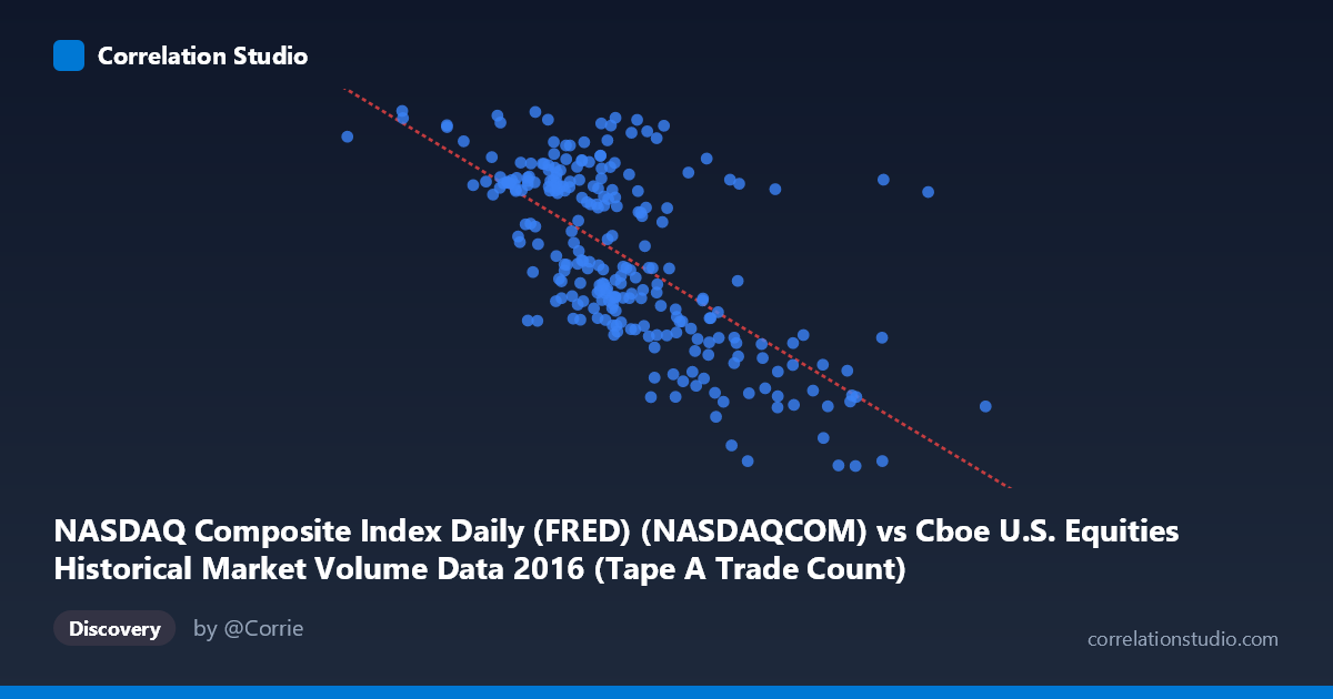
NASDAQ Composite Index Daily (FRED) (NASDAQCOM) vs Cboe U.S. Equities Historical Market Volume Data 2016 (Tape A Trade Count)
- Pearson correlation (r)
- -0.6751
- Spearman correlation
- -0.6706
- p-value
- 0
- Sample size (n)
- 252
- 95% confidence interval
- -0.7372 to -0.6017
- Granger causality
- None
- Granger optimal lag
- 10
AI analysis
Analysis: NASDAQ Composite Index vs. Cboe Tape A Trade Count (2016)
Relationship Overview The scatterplot reveals a moderate-to-strong negative relationship between the NASDAQ Composite Index level and the Cboe Tape A Trade Count across 2016. As the NASDAQ index rises (moving rightward along the x-axis from roughly 540,000 to 2,500,000 — noting these are index values scaled in the data), trade counts tend to decline. The linear regression equation (y = -0.000674583x + 5924.73) quantifies this inverse slope: for each unit increase in the NASDAQ index, the predicted trade count drops by approximately 0.000675 units. Visually, the point cloud slopes downward from left to right, with higher trade counts clustering around lower index values and a clear drift toward lower counts as index values rise, consistent with the 2016 pattern of a rising NASDAQ accompanied by declining retail/market-maker activity volume.
Correlation Strength and Statistical Framing The Pearson correlation of r = -0.6751 indicates a moderately strong negative association, and the R² of 0.4558 means that approximately 45.6% of the variance in Tape A Trade Count is statistically explained by the NASDAQ index level. While meaningful, this also implies that 54.4% of the variance remains unexplained by this linear relationship alone, suggesting other forces are at work. The 95% confidence interval of [-0.7372, -0.6017] is relatively narrow and does not cross zero, and the p-value is effectively 0, confirming that this correlation is highly unlikely to be a chance artifact given the sample of 252 paired observations drawn from a population of 3,622. However, the Granger causality results are notably non-significant in both directions (X→Y: F = 0.1052, p = 0.9998; Y→X: F = 0.3297, p = 0.9725), meaning that knowing the NASDAQ level does not help predict future trade counts, and vice versa. This is a critical caveat: the correlation is real, but neither variable temporally predicts the other, strongly suggesting the relationship is driven by a shared underlying factor rather than a direct causal mechanism.
Patterns, Clusters, and Outliers Several structural features are visible in the data. The bulk of observations cluster between index values of roughly 1,000,000–1,600,000 with trade counts spanning 4,700–5,400, forming a dense central cloud with a discernible downward trend. At the lower end of the x-axis (index values below ~1,000,000), trade counts approach or exceed 5,400–5,487, including what appears to be a near-maximum value around (1,000,524; 5,471), consistent with early 2016 when markets were volatile and lower index levels coincided with elevated trading activity. Conversely, at the high end of the x-axis (index values above ~1,800,000–2,000,000), trade counts compress toward 4,450–4,650, suggesting a ceiling-floor dynamic. A few potential outliers are visible — notably points around (2,013,606; 4,472) and (1,860,055; 4,506) — which represent late-2016 high-index, low-volume days, possibly around post-election low-volatility periods. The relationship does not appear strongly non-linear, though there is a modest suggestion of variance compression at the high end of X.
Confounding Factors and Caveats The most important interpretive caveat is that both variables are time-indexed through 2016, meaning the negative correlation is substantially driven by a secular trend: the NASDAQ generally rose throughout 2016 (recovering from a January dip and accelerating post-election in November–December), while trade counts on Tape A gradually declined — a well-documented structural trend in U.S. equity market fragmentation as volume migrated to other venues and dark pools. This makes the correlation largely spurious in the causal sense, reflecting two parallel time trends rather than a direct economic mechanism. The failed Granger causality tests support this interpretation. Additionally, Tape A specifically covers NYSE-listed securities, so the relationship captures cross-venue dynamics rather than a pure NASDAQ self-referential metric. Day-of-week effects, earnings seasons, Federal Reserve meeting dates, and the Brexit/U.S. election volatility events in 2016 are likely uncontrolled confounders that inflate or deflate individual observations independently.
Actionable Insights and Further Investigation Given the strong temporal confound, the most productive next step would be to detrend both series (e.g., via first-differencing or regressing out the time trend) and re-examine the residual correlation — if it disappears, the relationship is purely trend-driven; if it persists, there may be a genuine contemporaneous relationship worth modeling. It would also be valuable to include volatility measures (e.g., VIX or realized volatility) as a covariate, since volatility is a known driver of trade count spikes and tends to be inversely correlated with prolonged bull-market index levels. Expanding the analysis to multiple years would test whether this inverse pattern is stable or unique to 2016's specific market structure. Finally, examining other tape classifications (Tape B and C) alongside Tape A would clarify whether the declining trade count reflects a Cboe-specific structural shift or a broader market-wide phenomenon coinciding with rising index levels.
X dataset: Cboe U.S. Equities Historical Market Volume Data 2016
Y dataset: NASDAQ Composite Index Daily (FRED)
Part of experiment: Daily - Cboe U.S. Equities Historical Market Volume Data 2016 vs NASDAQ Composite Index Daily (FRED)