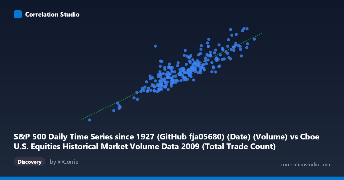
S&P 500 Daily Time Series since 1927 (GitHub fja05680) (Date) (Volume) vs Cboe U.S. Equities Historical Market Volume Data 2009 (Total Trade Count)
- Pearson correlation (r)
- 0.8738
- Spearman correlation
- 0.8501
- p-value
- 0
- Sample size (n)
- 252
- 95% confidence interval
- 0.841 to 0.9002
- Granger causality
- None
- Granger optimal lag
- 10
AI analysis
Analysis: S&P 500 Trading Volume vs. Cboe Total Trade Count (2009)
Relationship Overview The scatterplot reveals a strong positive linear relationship between S&P 500 daily trading volume and Cboe U.S. Equities total trade count across the 2009 trading year. As daily share volume increases, the total number of discrete trades rises proportionally, following the regression line y = 1920.45x + 4.51×10⁸ reasonably well across the observed range. This is intuitive: higher volume days naturally tend to involve more individual transactions, reflecting elevated market participation. The relationship spans a wide dynamic range — X values stretch from roughly 630K to 4.13M and Y from approximately 1.27B to 9.12B — suggesting the pattern holds across both quiet and highly active trading sessions.
Correlation Strength and Statistical Interpretation The Pearson correlation of r = 0.8738 indicates a strong positive association, and the R² of 0.7635 means that approximately 76.4% of the variance in total trade count is explained by trading volume alone. This is a practically meaningful result: volume is clearly a dominant driver of trade count, though roughly 23.6% of variance remains unexplained, attributable to other factors such as trade size distribution, fragmentation across venues, or algorithmic activity. The 95% confidence interval of [0.841, 0.900] is narrow and entirely positive, reinforcing high statistical reliability. The p-value of ~0 with n=252 drawn from a population of 3,232 leaves no credible doubt about the existence of a positive association. However, the Granger causality results are notably absent in both directions — X→Y (F=0.46, p=0.91) and Y→X (F=0.91, p=0.52) — meaning neither variable temporally predicts the other at the optimal 10-period lag. This is a critical caveat: despite the strong contemporaneous correlation, these variables move together rather than one leading the other, suggesting they are co-driven by common market forces rather than causally linked in sequence.
Patterns, Clusters, and Outliers The bulk of observations cluster in a moderately dense band roughly between X = 2.0M–3.5M and Y = 4.5B–7.5B, representing typical 2009 trading days. A few notable features stand out. At the lower-left extreme sits an apparent outlier near (629K, 1.27B), likely corresponding to an unusually quiet session (possibly a holiday-adjacent day). At the upper-right, points near (3.91M, 9.12B) and (4.13M, 8.21B) represent peak-activity sessions. There is also some vertical scatter at similar X values — for example, observations around X ≈ 2.1–2.2M show Y values ranging from roughly 4.1B to 6.3B — indicating that equivalent volume levels can correspond to meaningfully different trade counts depending on average trade size. This heteroscedasticity (scatter widening slightly at higher volumes) is mild but worth noting.
Confounding Factors and Caveats Several important caveats apply. First, 2009 was an extraordinary market year, encompassing the tail of the financial crisis, the March 2009 market bottom, and a dramatic recovery — regime changes that could inflate the apparent correlation by compressing unusual high-volatility/high-volume periods together. Second, the datasets come from different sources (Yahoo Finance S&P 500 data vs. Cboe market data), and any date-alignment mismatches or differing definitions of "volume" could introduce noise. Third, trade fragmentation — the proliferation of dark pools and alternative trading venues in 2009 — means Cboe trade count may not represent total market activity uniformly across the year. Finally, the lack of Granger causality confirms this is a concurrent, not predictive relationship, so using one variable to forecast the other in a time-series context would be unreliable.
Actionable Insights and Further Investigation Practitioners should treat this correlation as evidence of co-movement rather than a forecasting tool. To deepen understanding, several follow-up analyses are warranted: (1) Decompose residuals to identify which sessions deviate most from the regression line and investigate whether those correspond to specific market events (FOMC announcements, earnings seasons, crisis episodes); (2) Segment by market regime (pre/post March 9, 2009 bottom) to test whether the correlation strength differs across bull and bear phases; (3) Add average trade size as a third variable to explain the residual 23.6% variance, since volume ÷ trade count directly yields this metric; (4) Extend to multiple years to test whether the 2009 relationship is stable or an artifact of crisis-era conditions. The strong R² makes volume a useful contemporaneous proxy for market activity complexity, but the Granger results caution firmly against any causal or leading-indicator interpretation.
X dataset: Cboe U.S. Equities Historical Market Volume Data 2009
Y dataset: S&P 500 Daily Time Series since 1927 (GitHub fja05680) (Date)
Part of experiment: Daily - Cboe U.S. Equities Historical Market Volume Data 2009 vs S&P 500 Daily Time Series since 1927 (GitHub fja05680) (Date)