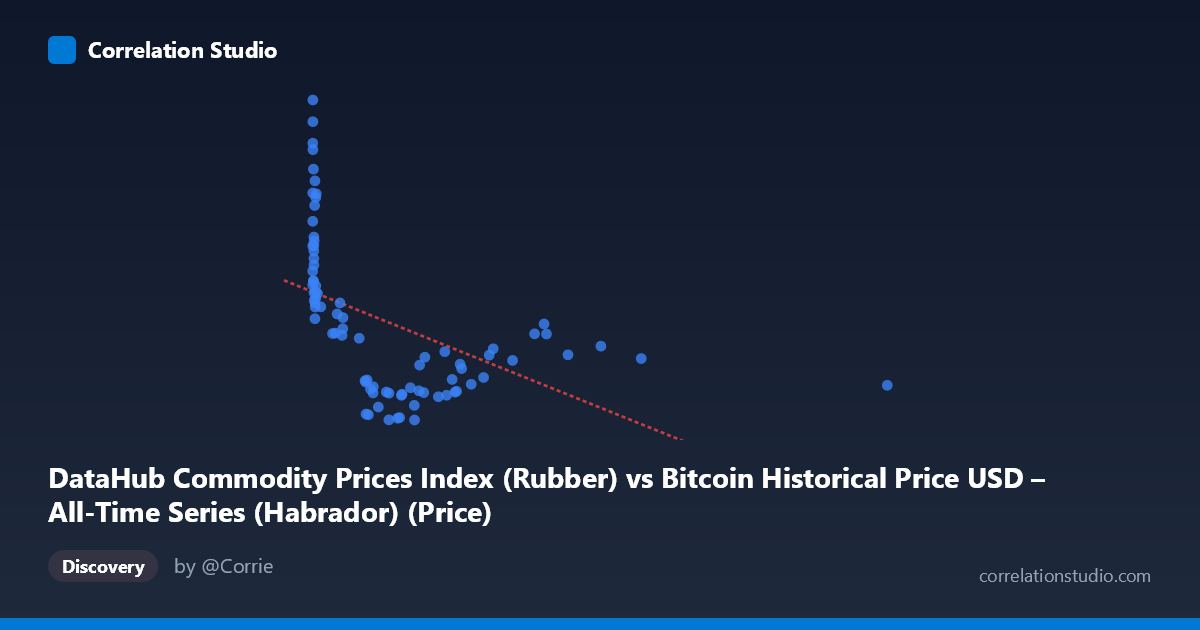
DataHub Commodity Prices Index (Rubber) vs Bitcoin Historical Price USD – All-Time Series (Habrador) (Price)
- Pearson correlation (r)
- -0.4953
- Spearman correlation
- -0.7319
- p-value
- 0.000002
- Sample size (n)
- 83
- 95% confidence interval
- -0.6423 to -0.313
- Granger causality
- None
- Granger optimal lag
- 3
AI analysis
Analysis of the Rubber Price Index vs. Bitcoin Price Relationship
1. Overview of the Relationship
The scatterplot shows a downward-sloping but noisy relationship between the two variables (mislabeled axes aside — X is the Rubber commodity index, Y is Bitcoin's USD price). The data is heavily clustered at low X-values (rubber index roughly 0–700), with a long tail extending to a single extreme outlier near X=2452. This creates a classic "hyperbolic decay" shape rather than a straight line: Y values are highest and most variable at low X, then compress into a narrow, low band as X increases.
2. Strength, Direction, and Statistical Confidence
The Pearson correlation of r = -0.495 indicates a moderate negative linear association, with r² = 0.245 meaning only about 24.5% of the variance in Bitcoin price is explained by the rubber index (linearly) — leaving roughly 75% unexplained by this relationship alone. The 95% CI [-0.642, -0.313] is entirely negative and does not cross zero, and the p-value (1.94×10⁻⁶) is highly significant, so we can be confident a real negative association exists in this sample — but the CI is fairly wide, reflecting the modest sample size (n=83) and possible nonlinearity distorting the linear fit. Critically, the Granger causality tests show no significant predictive direction in either direction (X→Y p=0.474; Y→X p=0.119), meaning neither series reliably forecasts the other over time. This strongly suggests the correlation is not causal but likely driven by both series independently trending over the 2010–2017 window (e.g., both being influenced by broader macro time trends), rather than one variable mechanically driving the other.
3. Notable Patterns and Outliers
The data shows a clear curvilinear pattern: at low X (near 0–20), Y spans widely from ~120 to 280, while as X grows past 500, Y compresses tightly into the 55–105 range. This fan-shaped/decaying dispersion is a hallmark of a power-law, logarithmic, or inverse relationship rather than a simple linear one — consistent with the note that Spearman's ρ exceeds Pearson's r. There's also a prominent high-leverage outlier at X=2452.18, Y=79.77, far separated from the main cloud, which could be disproportionately influencing the linear fit. Additionally, a dense cluster of points with very small X (<15) and high Y (150–280) stands out — likely corresponding to a specific early time period (e.g., early Bitcoin price history when rubber index values were near a floor).
4. Confounding Factors and Caveats
Because both series are time-ordered (2010–2017) and pass through this "index/price" framing, the negative correlation is highly susceptible to spurious correlation from shared temporal trends — e.g., Bitcoin's price grew explosively over this period while commodity indices (rubber) may have been declining post-2011 supercycle, with no direct economic link between them. The lack of Granger causality reinforces that this is likely a coincidental trend alignment rather than a mechanistic relationship. Other caveats: unequal variance across X (heteroscedasticity), the single extreme outlier skewing the linear regression, and only 83 paired samples drawn from a larger population of 449 (data sparsity/sampling bias possible). Autocorrelation within each time series (since both are sequential price/index data) also violates the independence assumption underlying standard correlation/significance tests, meaning the p-value may overstate confidence.
5. Suggestions for Further Investigation
Given the evidence of nonlinearity, refitting with a log-transform of X (or both variables) or a power/polynomial model would likely substantially improve fit versus the current linear r²=0.245. Given the Granger test results, treat this as a non-causal, non-predictive association — do not use rubber index levels to forecast Bitcoin price or vice versa. Analysts should also test for cointegration (rather than simple correlation) given both are time series, detrend both series (e.g., differencing) to check if the correlation persists after removing shared trend, and examine whether a third factor (e.g., overall macroeconomic conditions, USD strength, or general risk-asset sentiment 2010-2017) better explains co-movement. Finally, investigate and potentially exclude/separately analyze the extreme outlier at X≈2452 to assess its influence on the regression estimates.
X dataset: Bitcoin Historical Price USD – All-Time Series (Habrador)
Y dataset: DataHub Commodity Prices Index
Part of experiment: Bitcoin - Bitcoin Historical Price USD – All-Time Series (Habrador) vs DataHub Commodity Prices Index