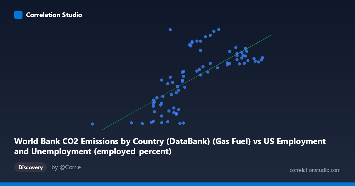
World Bank CO2 Emissions by Country (DataBank) (Gas Fuel) vs US Employment and Unemployment (employed_percent)
- Pearson correlation (r)
- 0.718
- Spearman correlation
- 0.7482
- p-value
- 0
- Sample size (n)
- 80
- 95% confidence interval
- 0.5917 to 0.81
- Granger causality
- None
- Granger optimal lag
- 10
AI analysis
Scatterplot Analysis: Gas Fuel CO2 Emissions vs. US Employment Percentage
1. Overall Relationship and Visualization
The scatterplot reveals a positive association between gas fuel CO2 emissions (X-axis, measured in units consistent with World Bank DataBank reporting) and the US employed percentage (Y-axis). As gas fuel CO2 emissions increase from roughly 50.4 to 64.4 units, employed percentage tends to rise from the low hundreds to values approaching 17,000 — a dramatic range. The linear regression equation (y = 1175.11x − 60,468.4) captures the general upward trend, but the scatter around this line is substantial, suggesting the relationship is real but far from deterministic. Visually, the data points fan outward at higher X values, hinting at heteroscedasticity and possible non-linear structure.
2. Correlation Strength, Direction, and Causality
The Pearson correlation of r = 0.718 indicates a moderately strong positive relationship, but the explanatory power is more sobering: R² = 0.516, meaning gas fuel CO2 emissions statistically explain only about 52% of the variance in employed percentage, leaving nearly half the variation unexplained by this model alone. The 95% confidence interval for r [0.592, 0.810] is reasonably tight and excludes zero, and the p-value of 6.55 × 10⁻¹⁴ confirms this correlation is overwhelmingly unlikely to be a chance artifact at any conventional significance threshold. However, the Granger causality analysis yields no significant directional predictive relationship in either direction — neither X→Y (F = 0.679, p = 0.739) nor Y→X (F = 1.366, p = 0.224) — meaning that past values of one variable do not significantly help predict future values of the other beyond each variable's own history. This is a critical caveat: statistical correlation exists, but temporal predictive causality does not, at least at the optimal 10-period lag tested.
3. Notable Patterns, Clusters, and Outliers
Several features stand out upon closer inspection:
- Lower X cluster (50–55 range): Points in this zone show uniformly low Y values (below ~5,000), with little spread, suggesting a floor effect or threshold behavior. - Middle X cluster (55–59): This region displays enormous vertical spread, with Y values ranging from below 1,000 to above 16,000 at nearly identical X values (e.g., multiple points near X = 57.8 span from ~829 to ~9,602). This variance explosion is the dominant source of unexplained R². - Upper X cluster (60–65): Points converge toward a moderate Y band (~10,000–17,000), with less scatter than the middle range, suggesting a possible ceiling or saturation effect. - Candidate outliers: The point (56.8, 16,953.61) stands dramatically above its X-neighborhood peers; similarly, (60.8, 16,992.26) and (60.1, 15,999.24) are notably high. At the low end, (50.4, 654.44) and (57.9, 829.71) anchor the floor. These outliers disproportionately influence regression slope and R².
The middle-range scatter strongly implies a non-linear or threshold relationship may better describe the data than a simple linear model.
4. Confounding Factors and Interpretive Caveats
Several important caveats apply before drawing any meaningful conclusions:
- Spurious correlation via shared time trend: Both gas fuel CO2 emissions and US employment percentage are annual time-series spanning 1941–2020. Both variables likely share upward secular trends driven by economic growth, population increase, and industrialization, making temporal co-movement almost inevitable without detrending. - Dataset mismatch / label confusion: The metadata raises a red flag — the X-axis variable is labeled as coming from "US Employment and Unemployment" data, yet it measures CO2 gas emissions, while the Y-axis is labeled as coming from "World Bank CO2 Emissions" yet measures employment percentage. This cross-dataset labeling inconsistency suggests possible data join errors that could introduce systematic noise or spurious structure. - Aggregation level: World Bank CO2 data is global/country-level; US employment is a national labor market indicator. Mixing these without controlling for country, GDP, or sectoral composition introduces significant confounding. - Omitted variables: Business cycles, oil price shocks, energy policy shifts, recessions (2008, COVID-era), and technological transitions all independently drive both emissions and employment, acting as common causes that inflate observed correlation. - Heteroscedasticity: The variance in Y clearly increases with X, violating OLS assumptions and potentially inflating or deflating confidence in specific fitted values.
5. Actionable Insights and Further Investigation
Despite the statistically significant correlation, the absence of Granger causality and the substantial unexplained variance call for a more rigorous analytical approach:
- Detrend both series (e.g., first-differencing or HP filter) before computing correlation to distinguish genuine co-movement from shared secular drift. - Investigate the outliers explicitly — the points with very high Y at mid-range X (e.g., 56.8, 16,953) may represent specific historical episodes (post-WWII boom, 1990s expansion) worth identifying and contextualizing. - Test non-linear models (polynomial, piecewise, or logarithmic regression) given the apparent threshold behavior below X ≈ 55 and saturation above X ≈ 60. - Resolve the dataset labeling discrepancy before any policy or research conclusions are drawn — the column-dataset attribution inconsistency must be verified as a metadata artifact or a genuine data join error. - Introduce control variables (GDP growth, oil prices, sectoral employment shares) in a multivariate framework to isolate any genuine partial correlation between energy use and employment outcomes. - Extend Granger causality testing across a range of lags (not just lag 10) and consider Vector Autoregression (VAR) modeling to more thoroughly characterize temporal dynamics.
Bottom line: The moderate-to-strong correlation (r = 0.718) is statistically robust but likely reflects shared macroeconomic and temporal trends rather than a direct causal mechanism. The lack of Granger causality, substantial mid-range scatter, and dataset labeling concerns collectively argue for treating this correlation as a hypothesis-generating finding rather than actionable evidence of a real-world mechanism.
X dataset: US Employment and Unemployment
Y dataset: World Bank CO2 Emissions by Country (DataBank)
Part of experiment: Yearly - US Employment and Unemployment vs World Bank CO2 Emissions by Country (DataBank)