Europe Brent Spot Price FOB Daily (Europe Brent Spot Price FOB (Dollars per Barrel)) vs Cboe U.S. Equities Historical Market Volume Data 2015 (Tape B Trade Count)
- Pearson correlation (r)
- -0.4573
- Spearman correlation
- -0.516
- p-value
- 0
- Sample size (n)
- 251
- 95% confidence interval
- -0.55 to -0.3535
- Granger causality
- None
- Granger optimal lag
- 1
AI analysis
Analysis: Europe Brent Spot Price vs. Cboe Tape B Trade Count (2015)
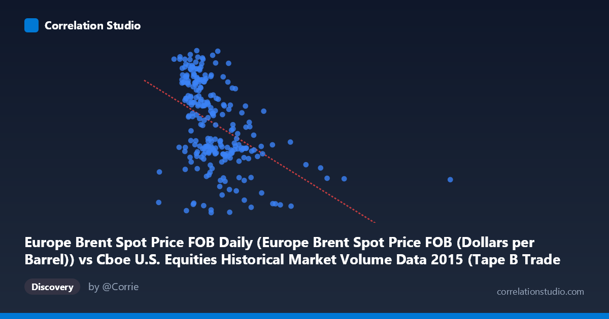
Relationship Overview The scatterplot reveals a negative relationship between Europe Brent crude oil spot prices (X-axis, dollars per barrel) and Cboe Tape B trade counts (Y-axis). As oil prices increase, trade counts tend to decline, and conversely, lower oil prices are associated with higher trading activity. The linear regression equation (y = -3.907×10⁻⁵x + 63.998) confirms this inverse trend, though the scatter around the regression line is substantial, indicating considerable unexplained variability. Notably, the bulk of observations cluster in the X range of roughly $130,000–$450,000 (in the dataset's units), with a long right tail of higher-price outliers that appear to anchor the negative slope.
Correlation Strength and Statistical Significance The Pearson correlation of r = -0.457 indicates a moderate negative association, but the coefficient of determination (r² = 0.209) reveals that only 20.9% of the variance in Tape B trade counts is explained by Brent oil prices — meaning roughly 79% of the variation remains unexplained by this relationship alone. The 95% confidence interval of [-0.550, -0.354] is entirely negative, confirming the direction is consistent, and the p-value of 2.24×10⁻¹⁴ establishes high statistical significance given the sample of 251 paired observations drawn from a population of 3,302. However, statistical significance here is partly a function of sample size and should not be conflated with practical or economic importance. Critically, the Granger causality tests fail in both directions (X→Y: F=1.27, p=0.260; Y→X: F=1.35, p=0.247), meaning neither variable demonstrates statistically meaningful temporal predictive power over the other at a 1-period lag. This absence of Granger causality strongly cautions against interpreting the correlation as reflecting any directional or mechanistic relationship.
Patterns, Clusters, and Outliers The data exhibit a dense primary cluster concentrated between approximately $130,000–$400,000 on the X-axis and 43–66 on the Y-axis, where the negative trend is most visible. Within this cluster, there is notable vertical spread at any given price level, suggesting high day-to-day variability in trade counts independent of oil price. Several high-price outliers (e.g., points near $621,000 and $640,000 with Y values around 41–44) sit far to the right and appear to exert leverage on the regression slope, potentially amplifying the apparent negative correlation. A handful of points also show elevated trade counts (above 62–66) paired with relatively low oil prices, forming a distinct upper-left grouping that reinforces the inverse pattern but may reflect episodic volatility events rather than a systematic relationship.
Confounding Factors and Caveats Several important caveats apply. First, 2015 was an extraordinary year for oil markets, marked by a dramatic price collapse driven by OPEC supply decisions and global oversupply — this structural break means the time series captures a highly unusual regime rather than typical dynamics. Second, Tape B trade counts reflect activity on specific U.S. regional exchanges and are influenced by market microstructure factors (routing decisions, venue competition, ETF rebalancing, algorithmic activity) that have no direct connection to commodity prices. Third, the correlation may be spurious or mediated by a common driver — for example, broad market volatility (VIX) rising during the oil sell-off could simultaneously suppress oil prices and alter exchange-specific routing patterns. Finally, the long right tail in X (max ~$1,014,000 versus mean ~$299,000) suggests possible data scaling issues or outliers that warrant verification before drawing firm conclusions.
Actionable Insights and Further Investigation Given the moderate but mechanistically unexplained correlation and absent Granger causality, several next steps are warranted. Controlling for market-wide volatility (e.g., including VIX or total market volume as covariates) would help determine whether the oil-trade count relationship survives as an independent signal or dissolves into a broader risk-appetite story. Analysts should test longer lag structures in the Granger framework (beyond 1 period) and examine whether the relationship holds across other years to assess its robustness outside the 2015 oil crash regime. Decomposing the X variable to separate the oil price level from its rate of change (daily returns) may reveal whether it is price momentum rather than price level that drives trading behavior. Finally, comparing Tape B specifically against Tape A and C volumes would clarify whether this pattern is idiosyncratic to one exchange segment or reflects a market-wide phenomenon.
X dataset: Cboe U.S. Equities Historical Market Volume Data 2015
Y dataset: Europe Brent Spot Price FOB Daily
Part of experiment: Daily - Cboe U.S. Equities Historical Market Volume Data 2015 vs Europe Brent Spot Price FOB Daily