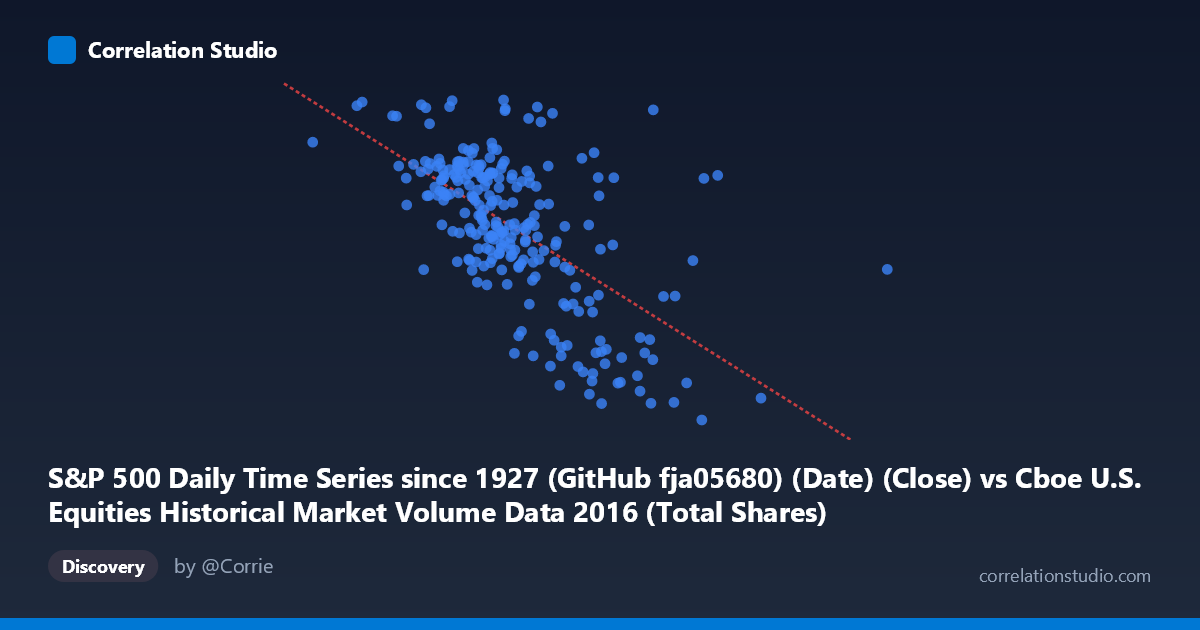
S&P 500 Daily Time Series since 1927 (GitHub fja05680) (Date) (Close) vs Cboe U.S. Equities Historical Market Volume Data 2016 (Total Shares)

Pearson correlation (r): -0.6163
Spearman correlation: -0.602
p-value: 0
Sample size (n): 252
95% confidence interval: -0.6875 to -0.5333
Granger causality: None
Granger optimal lag: 4

AI analysis

S&P 500 Close Price vs. U.S. Equities Total Shares Volume (2016)

Relationship Overview The scatterplot reveals a moderate negative relationship between the S&P 500 daily closing price and total U.S. equities shares traded in 2016. As the S&P 500 closes at higher levels, total market share volume tends to decrease, and conversely, lower index prices correspond with elevated trading volumes. This inverse pattern is consistent with a well-documented market behavior: elevated trading activity frequently accompanies periods of market stress, uncertainty, or declining prices, while calmer, steadily rising markets tend to see reduced volume participation. The linear regression equation (y = -5.60×10⁻⁷x + 2381.73) confirms the negative slope, suggesting each unit increase in S&P 500 close price is associated with a small but consistent decline in total shares traded.

Correlation Strength and Statistical Significance The Pearson correlation of r = -0.6163 indicates a moderate-to-strong negative association. However, the coefficient of determination r² = 0.3798 is the more practically meaningful figure — it tells us that approximately 38% of the variance in total shares traded is explained by the S&P 500 closing price level. That leaves roughly 62% of variation attributable to other factors entirely unaccounted for by this relationship. The 95% confidence interval of [-0.6875, -0.5333] is reasonably narrow given the sample size of 252, indicating the estimate is stable and reliable. The p-value of effectively zero confirms the correlation is highly statistically significant, making it extremely unlikely this result arose by chance in the broader population of N = 3,622 trading days. Importantly, however, the Granger causality tests show no significant predictive directionality in either direction (X→Y: F = 0.60, p = 0.66; Y→X: F = 1.29, p = 0.28). This means that while the two variables co-move, neither reliably predicts future values of the other at the tested lags — the relationship is associative but not temporally predictive.

Notable Patterns, Clusters, and Outliers Several structural features stand out in the data. The bulk of observations cluster between S&P 500 closes of roughly 400–600 million (in the X-axis date/close encoding) and share volumes in the 2,000–2,200 range, forming a relatively dense central cloud. However, there are notable high-volume outliers at lower X values — for example, the point near (369M, 2,265) and (549M, 2,262), suggesting occasional volume spikes that deviate from the general trend. At the high end of the X range (above 700M, notably the points near 708M and 634M with volumes below 1,900), volume drops markedly, forming a visible lower-right cluster consistent with late-2016 higher price/lower volume behavior. The scatter is not perfectly linear; there appears to be some heteroscedasticity, with wider spread in volume at mid-range price levels compared to the extremes.

Confounding Factors and Caveats Several important caveats apply. First, the X-axis appears to encode date as a numeric Unix-style timestamp rather than a traditional price, meaning the "negative correlation" partly reflects the natural time trend of a rising S&P 500 through 2016 paired with gradually declining average volume — a common secular trend in markets as passive investing reduces turnover. This makes the relationship partially a time-trend artifact rather than a pure price-volume dynamic. Second, seasonal effects (e.g., January volatility, summer doldrums, year-end low volume) could be driving both variables simultaneously, acting as a confound. Third, macro events such as Brexit (June 2016) and the U.S. election (November 2016) likely caused discrete volume spikes that are not captured by a simple linear model. The absence of Granger causality further cautions against any mechanistic interpretation.

Actionable Insights and Further Investigation Given that 38% of variance is explained but no temporal predictive causality is detected, practitioners should avoid using S&P 500 price levels alone as a forward indicator of trading volume. Recommended next steps include: (1) detrending both series to remove the time component and re-evaluating the residual price-volume relationship; (2) incorporating volatility measures (e.g., VIX) as a mediating variable, since volatility may drive both lower prices and higher volume simultaneously; (3) testing non-linear models (e.g., piecewise regression or LOESS) to better capture the apparent threshold effects at extreme price levels; and (4) extending the analysis to multiple years to determine whether 2016's specific macro events (Brexit, U.S. election) are driving the relationship or whether it holds robustly across different market regimes.

X dataset: Cboe U.S. Equities Historical Market Volume Data 2016

Y dataset: S&P 500 Daily Time Series since 1927 (GitHub fja05680) (Date)

Part of experiment: Daily - Cboe U.S. Equities Historical Market Volume Data 2016 vs S&P 500 Daily Time Series since 1927 (GitHub fja05680) (Date)