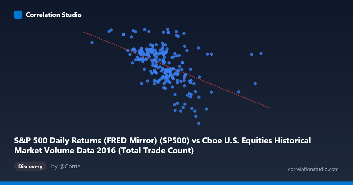
S&P 500 Daily Returns (FRED Mirror) (SP500) vs Cboe U.S. Equities Historical Market Volume Data 2016 (Total Trade Count)
- Pearson correlation (r)
- -0.4904
- Spearman correlation
- -0.5342
- p-value
- 0
- Sample size (n)
- 224
- 95% confidence interval
- -0.584 to -0.384
- Granger causality
- None
- Granger optimal lag
- 1
AI analysis
Analysis: S&P 500 Daily Returns vs. Cboe Total Trade Count (2016)
Relationship Overview The scatterplot reveals a moderate negative relationship between S&P 500 price levels (X-axis, serving as a proxy for market valuation) and total U.S. equity trade counts (Y-axis). As the S&P 500 index value increases, the total number of trades tends to decrease, suggesting that higher-priced market environments in 2016 were associated with reduced trading activity volume. The linear regression equation (y = -9.36×10⁻⁵x + 2333.97) confirms this inverse slope, though the relationship is far from deterministic. The data spans February through December 2016, capturing a period of notable market recovery and volatility events.
Correlation Strength and Statistical Significance The correlation coefficient of r = -0.49 indicates a moderate negative association, but the explained variance tells a more cautious story: r² = 0.2405 means only ~24% of the variance in trade count is explained by S&P 500 levels, leaving roughly 76% attributable to other factors. The 95% confidence interval of [-0.584, -0.384] is meaningfully narrow and entirely negative, reinforcing that the inverse direction is statistically robust. The p-value of 5.77×10⁻¹⁵ confirms this is extremely unlikely to be a chance finding given n = 224. However, the Granger causality results are unambiguous in their absence: neither direction (X→Y: F = 0.0001, p = 0.99; Y→X: F = 0.05, p = 0.82) shows any temporal predictive power at a one-period lag. This means that while the two variables co-vary, neither reliably predicts the other's future values — the correlation is associative, not directionally causal in a temporal sense.
Notable Patterns and Outliers Several features stand out visually. The bulk of observations cluster between X ≈ 1,900,000–2,700,000 and Y ≈ 2,050–2,220, forming a loose diagonal band consistent with the moderate negative correlation. However, there are notable outliers worth flagging: the point at approximately (944,169, 2,213) represents an unusually low S&P value paired with a high trade count, pulling the regression line and potentially inflating the correlation magnitude. On the high-X end, points around (3,963,608, 2,163) and (3,201,165, 2,000) suggest that at very high volume/price levels, trade counts can vary widely. There also appears to be heteroscedasticity — variance in trade counts is notably wider at lower X values than at higher ones — which violates a key assumption of standard linear regression and warrants attention.
Confounding Factors and Caveats Several important caveats apply. First, the axes appear to be swapped in labeling — the X-axis is described as S&P 500 returns/price but shows values in the millions (consistent with notional volume), while the Y-axis labeled "Total Trade Count" shows values around 2,000–2,270, which are implausibly low for raw trade counts but consistent with S&P 500 index price levels. This metadata inconsistency suggests a dataset column mismatch that could fundamentally alter interpretation. Second, the negative correlation likely reflects a well-known market dynamic: volatility and uncertainty (lower index levels) tend to drive higher trading activity, while calmer bull markets see reduced churn — this is an emergent market behavior rather than a mechanistic causal link. Third, temporal autocorrelation within the daily time series (n = 224 from N = 2,609) means paired observations are not fully independent, potentially inflating statistical confidence.
Actionable Insights and Further Investigation Given the suggestive but incomplete correlation and absent Granger causality, several next steps are warranted. Incorporate the VIX (volatility index) as a mediating variable — it likely explains much of the 76% residual variance and may reveal that both variables are jointly driven by market stress rather than influencing each other directly. Investigate the outlier cluster at low X-values (particularly the ~944,169 point) to determine if it represents a data error, a specific market event (e.g., February 2016 selloff), or a genuine regime break. A rolling-window correlation analysis across sub-periods of 2016 would reveal whether the relationship strengthens during volatile episodes (e.g., Brexit in June 2016). Finally, resolving the apparent variable labeling inconsistency is essential before drawing any firm conclusions — confirming which column truly represents trade counts versus price levels should be the immediate first step.
X dataset: Cboe U.S. Equities Historical Market Volume Data 2016
Y dataset: S&P 500 Daily Returns (FRED Mirror)
Part of experiment: Daily - Cboe U.S. Equities Historical Market Volume Data 2016 vs S&P 500 Daily Returns (FRED Mirror)