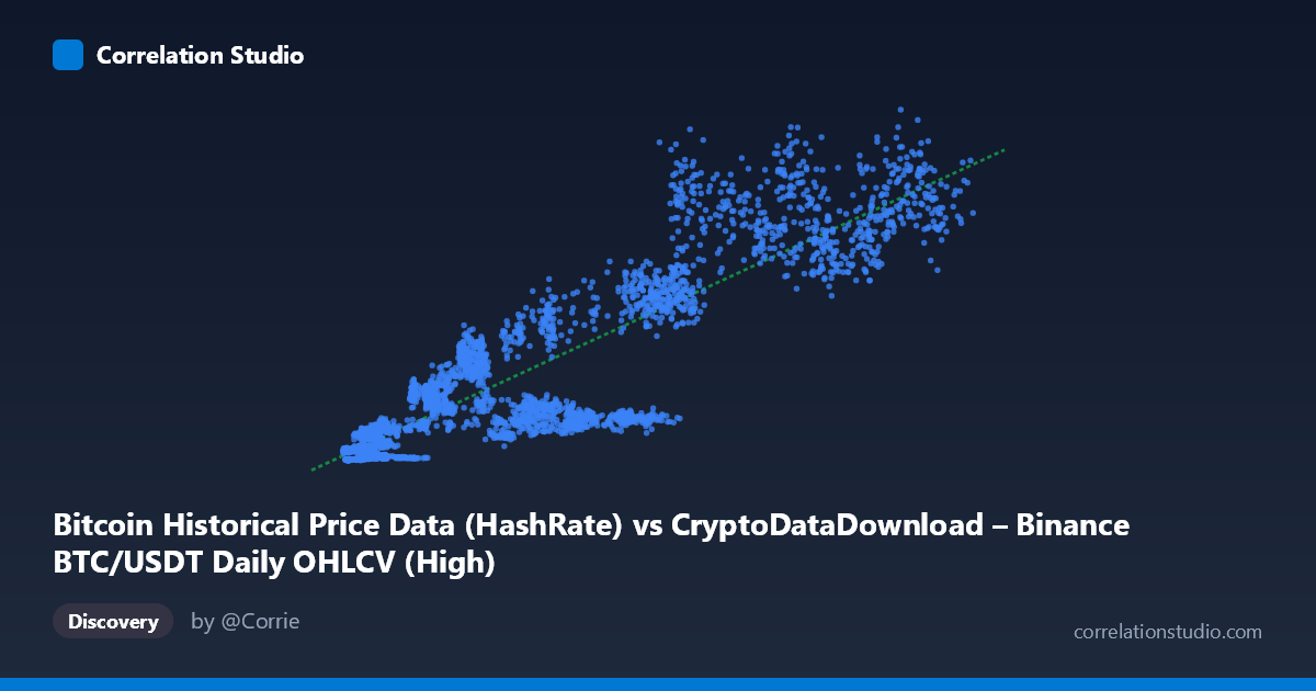
Bitcoin Historical Price Data (HashRate) vs CryptoDataDownload – Binance BTC/USDT Daily OHLCV (High)
- Pearson correlation (r)
- 0.8894
- Spearman correlation
- 0.88
- p-value
- 0
- Sample size (n)
- 3191
- 95% confidence interval
- 0.8819 to 0.8964
- Granger causality
- None
- Granger optimal lag
- 10
- Time coverage
- 2017-08-17 to 2026-05-20
AI analysis
Analysis: Bitcoin Hash Rate vs. Price Relationship
1. What the Visualization Reveals
The scatterplot displays a strong, positive, monotonic relationship between the X variable (labeled "HashRate" but populated with values in the thousands—likely a proxy metric or mislabeled field) and Y (BTC/USDT daily high price). As X increases from roughly 3,300 to 126,000, Y climbs from single-digit millions to over 1.3 billion, suggesting these are index or scaled values rather than raw hash rate (EH/s) and raw USD price. The overall shape is upward-sloping and reasonably linear, though with visible fanning/heteroscedasticity—variance in Y grows substantially as X increases, a common feature of financial and network-growth data.
2. Strength, Direction, and Statistical Confidence
The correlation is strong and positive (r = 0.889), with r² indicating that 79.1% of the variance in Y is statistically explained by X in a linear framework—leaving about 21% attributable to other factors, noise, or non-linear dynamics. The 95% CI [0.882, 0.896] is tight, reflecting the large sample size (n=3,191) and giving high confidence that this correlation is not a sampling artifact; the p-value of ~0 confirms the relationship is highly statistically significant.
However, correlation here does not imply directional causality. The Granger causality tests show no significant predictive direction in either direction (X→Y: p=0.47; Y→X: p=0.12) at the optimal 10-period lag. This means neither variable reliably "leads" the other in a time-series forecasting sense—despite their strong contemporaneous association, past values of one do not significantly improve prediction of future values of the other beyond what the variable's own history provides. This is a critical distinction: the two series likely move together because they're both driven by a common underlying trend (e.g., overall Bitcoin network/market growth over 2017–2026) rather than one mechanically causing the other.
3. Notable Patterns and Non-linear Features
Several features stand out: - Fanning/heteroscedasticity: at low X (<15,000), Y values cluster tightly in the tens of millions; at high X (80,000), Y spans hundreds of millions to over a billion, indicating increasing volatility at higher levels—typical of exponential or multiplicative growth processes. - Possible regime clustering: points like (56,757.91, 118,398,932) and (59,368, 158,693,646) sit noticeably below the regression line compared to neighboring X values with much higher Y, suggesting distinct market regimes or cycles (e.g., bear vs. bull market periods) where the same X level maps to very different Y outcomes. - Curvature: the relationship may be better fit by a power-law or log-log model rather than a strict line, given that Y spans nearly 5 orders of magnitude while X spans less than 2 orders of magnitude—consistent with Bitcoin's historical exponential price appreciation relative to network metrics.
4. Confounding Factors and Caveats
- Both variables are macro-trending time series: since both X and Y have grown persistently since 2017 (likely tracking Bitcoin's overall adoption and market cap growth), much of the correlation may be a spurious trend correlation—two unrelated-but-both-increasing series will show high r even without direct causal linkage. This is reinforced by the null Granger causality result. - Autocorrelation: daily financial/network data is highly autocorrelated; the "n=3,191" independent pairs assumption for significance testing is likely violated, meaning the true effective sample size (and thus true confidence in p-values) is smaller than reported. - Field ambiguity: X is labeled "HashRate" but sourced from an OHLCV price dataset column—this suggests a data pipeline or labeling error, and the actual variable being analyzed should be verified before drawing domain conclusions about hash rate's relationship to price. - Market regime effects: bull/bear cycles, halving events, and macro liquidity conditions could be common confounders driving both series independently.
5. Actionable Recommendations
1. Verify data provenance: confirm whether X truly represents hash rate or is mislabeled price/volume data, since the current axis description conflicts with the stated dataset column. 2. De-trend before modeling: apply differencing or detrending (e.g., % daily change) to both series and re-run correlation/Granger tests to check if the relationship holds after removing shared macro-trend effects—this will reveal whether a genuine short-term relationship exists. 3. Try log-log regression: given the multiplicative growth pattern, fit log(Y) ~ log(X) to better capture the non-linear scaling and likely improve model fit. 7. Segment by market regime: analyze correlation separately across bull/bear periods or halving cycles to check for regime-dependent relationship strength, given the fanning pattern observed.
X dataset: CryptoDataDownload – Binance BTC/USDT Daily OHLCV
Y dataset: Bitcoin Historical Price Data
Part of experiment: Bitcoin - CryptoDataDownload – Binance BTC/USDT Daily OHLCV vs Bitcoin Historical Price Data