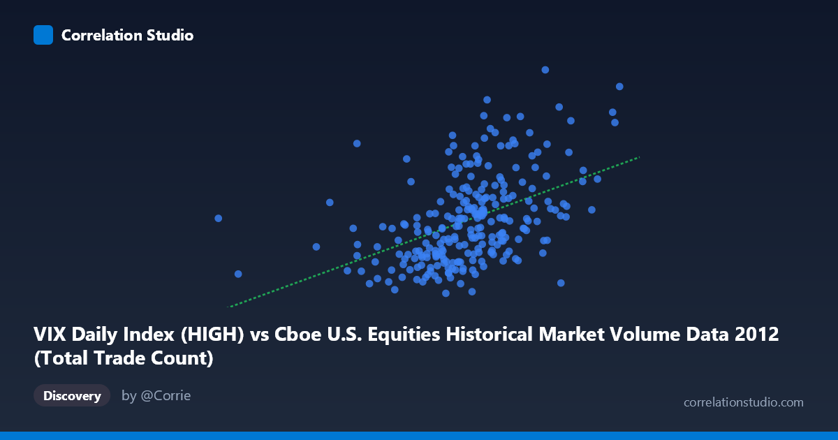
VIX Daily Index (HIGH) vs Cboe U.S. Equities Historical Market Volume Data 2012 (Total Trade Count)
- Pearson correlation (r)
- 0.4614
- Spearman correlation
- 0.5046
- p-value
- 0
- Sample size (n)
- 250
- 95% confidence interval
- 0.3578 to 0.5538
- Granger causality
- None
- Granger optimal lag
- 1
AI analysis
Analysis: VIX Daily Index (HIGH) vs. Total Trade Count — 2012
Relationship Overview
The scatterplot reveals a positive relationship between the VIX Daily Index High values and the Total Trade Count in U.S. equities markets during 2012. As VIX High readings increase, total trade counts tend to rise as well, which is intuitively consistent with market microstructure theory: elevated volatility typically drives higher trading activity as participants react to uncertainty, rebalance portfolios, and execute hedging strategies. The linear regression equation (y = 5.28E-06x + 9.89) captures this upward trend, though the scatter around the regression line is visibly substantial, signaling that the relationship, while real, is far from deterministic.
Correlation Strength and Statistical Significance
The Pearson correlation of r = 0.4614 indicates a moderate positive association. However, the more practically informative metric is r² = 0.2129, meaning that VIX High levels explain only about 21.3% of the variance in total trade counts — leaving nearly 79% of variation unexplained by this single predictor alone. The 95% confidence interval of [0.3578, 0.5538] is meaningfully above zero and reasonably tight given the sample size of 250, and the p-value of 1.40E-14 confirms the correlation is highly statistically significant, making it extremely unlikely to be a chance finding in this dataset. Despite statistical significance, however, the Granger causality analysis tells a more cautious story: neither direction (X→Y nor Y→X) reaches significance (F = 0.23, p = 0.63; F = 0.24, p = 0.62), meaning there is no evidence of temporal predictive directionality between the two series at a one-period lag. In practical terms, knowing today's VIX High does not reliably predict tomorrow's trade count, and vice versa — the correlation likely reflects contemporaneous co-movement rather than a leading-lagging relationship.
Notable Patterns, Clusters, and Outliers
Examining the sample points, several features stand out. The data exhibits a loose but discernible positive trend, with the bulk of observations clustering in the X range of roughly 1,400,000–1,900,000 and Y range of 15–22. There appear to be two loosely separated clusters: a denser lower-left grouping (lower VIX, lower trade counts) and a more dispersed upper-right grouping. A handful of notable outliers deserve attention — particularly points with high Y values (e.g., ~23–27) occurring at moderate X values around 1,550,000–1,750,000, suggesting that exceptionally high trade counts sometimes occur without correspondingly extreme VIX readings. Conversely, some high X values (approaching 2,000,000–2,200,000) are paired with only modest Y values (~14–19), indicating that heavy market volume does not always coincide with peak volatility. This asymmetry hints at non-linear or threshold dynamics that a simple linear fit may not adequately capture.
Confounding Factors and Interpretive Caveats
Several important caveats apply. First, axis labeling appears to be transposed in the dataset metadata — VIX values are described as the X-axis variable from a "market volume" dataset, while trade counts are attributed to the "VIX Daily Index" dataset, suggesting a potential data-joining or labeling artifact that should be verified before drawing firm conclusions. Second, the 2012 time window is a single-year snapshot following the European sovereign debt crisis, a period with its own idiosyncratic volatility regime, limiting generalizability. Third, algorithmic and high-frequency trading activity was a major driver of trade counts in 2012, which may respond to volatility spikes in ways decoupled from retail or institutional behavior. Fourth, seasonality and macroeconomic events (e.g., fiscal cliff concerns late in 2012) could simultaneously elevate both VIX and trade counts, creating spurious correlation through a common third driver.
Actionable Insights and Further Investigation
Given the moderate but incomplete explanatory power, several follow-up analyses are warranted. Introducing additional predictors — such as VIX Low, the VIX term structure (spread between near- and far-dated contracts), or market breadth indicators — could substantially improve variance explained. A non-linear regression or piecewise model should be tested, particularly to examine whether trade count responses to VIX accelerate beyond certain volatility thresholds (e.g., VIX 20). Rolling-window Granger causality at multiple lags (beyond just lag 1) would better characterize whether predictive relationships emerge over different time horizons. Finally, segmenting the data by exchange or trade type (e.g., separating TRF trades from lit exchange volume) could reveal heterogeneous dynamics masked in the aggregate, and extending the analysis across multiple years would determine whether the 2012 relationship is structurally stable or regime-dependent.
X dataset: Cboe U.S. Equities Historical Market Volume Data 2012
Y dataset: VIX Daily Index
Part of experiment: Daily - Cboe U.S. Equities Historical Market Volume Data 2012 vs VIX Daily Index