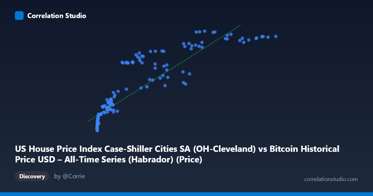
US House Price Index Case-Shiller Cities SA (OH-Cleveland) vs Bitcoin Historical Price USD – All-Time Series (Habrador) (Price)
- Pearson correlation (r)
- 0.8892
- Spearman correlation
- 0.9669
- p-value
- 0
- Sample size (n)
- 187
- 95% confidence interval
- 0.8548 to 0.9158
- Granger causality
- None
- Granger optimal lag
- 1
AI analysis
Analysis: Bitcoin Price vs. Cleveland Case-Shiller Home Price Index
1. What the Visualization Reveals
The scatterplot shows a strong, positive, and visibly non-linear relationship between Bitcoin's historical USD price and the Cleveland Case-Shiller Home Price Index. At low Bitcoin prices (under $1,000), the housing index clusters tightly between roughly 97–125, showing very little variation despite Bitcoin fluctuating across several orders of magnitude in this range. As Bitcoin prices climb into the tens of thousands and beyond, the housing index rises more steadily into the 140–205 range. This produces a curve that resembles a logarithmic or power-law relationship rather than a straight line — consistent with Bitcoin's price data spanning nearly six orders of magnitude (0.06 to 118,670) while the housing index only varies by about 2x.
2. Strength, Direction, and Statistical Uncertainty
The correlation coefficient (r = 0.889, r² = 0.791) indicates a strong positive association, with roughly 79% of the variance in the housing index statistically explained by Bitcoin price levels (or vice versa, since correlation doesn't specify direction). The 95% CI [0.855, 0.916] is tight and does not cross zero, and the p-value is effectively 0, meaning this correlation is highly unlikely to be a statistical fluke. However — and this is critical — the Granger causality tests show no significant predictive direction in either direction (X→Y: p=0.261; Y→X: p=0.138). This means neither variable's past values reliably help forecast the other's future values, despite the strong contemporaneous correlation. This is a textbook case where a robust correlation does not imply a lead-lag causal relationship — both series appear to be moving together due to a shared external driver (likely time/macro trend) rather than one causing the other.
3. Notable Patterns and Features
- Non-linear curvature: The relationship looks logarithmic in X — Bitcoin's early years (prices near $0) show enormous relative price swings while housing barely moves, then housing tracks Bitcoin's rise once BTC crosses ~$1,000. - Dense low-end cluster: Points with X < 1,000 dominate the sample count but occupy a narrow Y band (99–125), reflecting Bitcoin's early history (2010–2013) when housing was still recovering post-2008. - High-end acceleration: Above X ≈ 20,000, Y values climb quickly and become more scattered (e.g., 56,973 → 162.22 vs. 58,254 → 190.27), suggesting increased variance/noise at higher Bitcoin prices — possibly reflecting different market regimes (2017 bubble vs. 2020–2021 bull run vs. 2024–2025). - A few high-Y outliers at moderate X (e.g., 29,111.52 → 144.34, notably lower than neighboring points near 26,819–29,675 with Y in the high 170s–180s) suggest short-term decoupling, likely tied to specific calendar periods rather than price level itself.
4. Confounding Factors and Caveats
This is almost certainly a spurious or trend-driven correlation rather than a genuine economic relationship. Both series are strongly time-trending: Bitcoin has appreciated dramatically since 2010, and US home prices have risen steadily due to inflation, low interest rates (until 2022), and post-2008 recovery dynamics. When two independent time series both trend upward over the same 15+ year window, they will show strong correlation without any causal link. The lack of Granger causality supports this interpretation — it's consistent with "common trend" rather than "one drives the other." Additionally, comparing a highly volatile, globally-traded speculative asset (Bitcoin) to a regional, seasonally-adjusted, slow-moving housing index (single Ohio metro) is an unusual pairing with no clear economic mechanism connecting them directly.
5. Suggestions for Further Investigation
- Detrend both series (e.g., using differencing, or regressing out a time trend) and re-examine correlation on the residuals to check whether the relationship survives — this would be a stronger test for genuine linkage vs. shared drift. - Log-transform Bitcoin price (given its multi-order-of-magnitude range) before fitting a linear model; this would likely improve fit and better reflect the visible logarithmic curvature. - Introduce a proper macro control variable (e.g., CPI, M2 money supply, Fed funds rate) that could be the true common driver behind both series' long-term appreciation. - Treat this correlation as an artifact of the study period (2010–2026) rather than actionable investment or forecasting signal, especially given the null Granger causality result — this pairing should not be used to predict housing prices from Bitcoin trends or vice versa.
X dataset: Bitcoin Historical Price USD – All-Time Series (Habrador)
Y dataset: US House Price Index Case-Shiller Cities SA
Part of experiment: Bitcoin - Bitcoin Historical Price USD – All-Time Series (Habrador) vs US House Price Index Case-Shiller Cities SA