NASDAQ Composite Index Daily (FRED) (NASDAQCOM) vs Cboe U.S. Equities Historical Market Volume Data 2016 (Tape A Shares)
- Pearson correlation (r)
- -0.5945
- Spearman correlation
- -0.6135
- p-value
- 0
- Sample size (n)
- 252
- 95% confidence interval
- -0.6689 to -0.5083
- Granger causality
- None
- Granger optimal lag
- 10
AI analysis
Scatterplot Analysis: NASDAQ Composite Index vs. Cboe U.S. Equities Market Volume (2016)
Relationship Overview
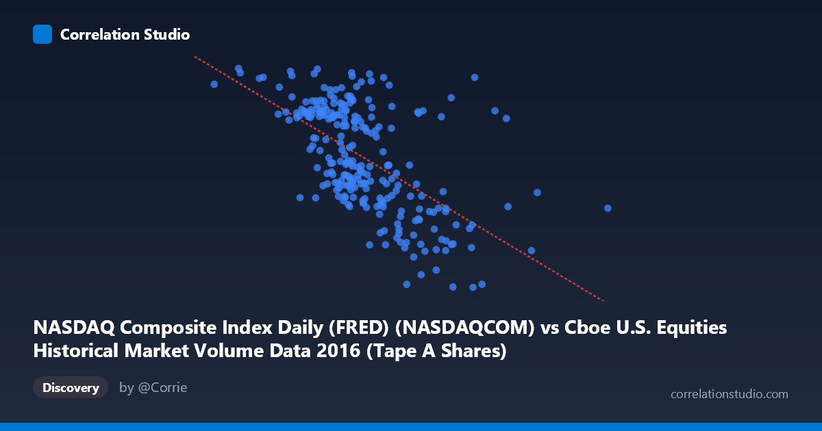
The scatterplot reveals a moderate negative relationship between the NASDAQ Composite Index daily closing value (X-axis) and Cboe U.S. Equities Tape A share volume (Y-axis) across 252 trading days in 2016. As the NASDAQ index climbed from roughly 105M to 543M units on the x-scale, Tape A share volume tended to decline — meaning that on days when equity valuations were higher, trading volume in Tape A shares was generally lower. This inverse pattern is visually apparent as a downward-sloping cloud of points, consistent with the fitted linear regression: y = -3.00253E-06x + 5805.97. The negative slope, while modest in absolute terms, captures a meaningful directional trend across the full trading year.
Correlation Strength and Statistical Significance
The Pearson correlation of r = -0.5945 indicates a moderate negative association, but the explanatory power is more modest than the r-value alone might suggest. The r² = 0.3534 means that only 35.3% of the variance in Tape A share volume is explained by the NASDAQ index level — leaving nearly two-thirds of the variation attributable to other factors. The 95% confidence interval of [-0.6689, -0.5083] is reassuringly narrow and does not cross zero, reinforcing that the negative direction is reliable. With a p-value effectively at zero and a sample of n = 252 drawn from a population of N = 3,622, the result is highly statistically significant and unlikely to be a sampling artifact. However, the Granger causality tests tell a more cautionary tale: neither direction (X→Y nor Y→X) achieves significance (F = 0.40, p = 0.94 and F = 0.67, p = 0.75 respectively), meaning that despite a robust contemporaneous correlation, neither variable temporally predicts the other at the optimal 10-period lag. This is an important distinction — correlation here does not translate into predictive or causal leverage.
Patterns, Clusters, and Outliers
Visually, the data cloud is widest in the mid-range of X (roughly 220M–310M), where considerable vertical scatter exists — Tape A volume ranges from approximately 4,500 to 5,500 in this zone, suggesting substantial day-to-day noise even at typical index levels. At the lower end of the X range (index levels below ~200M), several points cluster at notably high Tape A volumes (5,200–5,490), including the point at approximately (176.9M, 5,232) and (190.3M, 5,471) — these likely correspond to early 2016 market stress periods when lower valuations coincided with elevated trading activity, a classic fear-driven volume spike. Conversely, at higher index values (above ~330M), volume tends to compress toward 4,400–4,600, with the point near (363M, 4,472) standing as a notable high-index/low-volume anchor. There is no strong evidence of non-linearity, though the relationship may tighten slightly at the extremes.
Confounding Factors and Caveats
Several important caveats limit causal interpretation. First, time ordering matters: 2016 began with significant market volatility (early January selloff) and ended with a post-election rally, meaning the negative correlation partly reflects a temporal confound — early-year low prices coinciding with high-anxiety volume, and late-year high prices coinciding with calmer, lower-volume trading. This secular trend could manufacture correlation without any structural relationship between index level and volume. Second, Tape A specifically covers NYSE-listed securities, not NASDAQ-listed ones, making a direct mechanistic link to the NASDAQ Composite somewhat indirect. Third, macroeconomic events (Brexit vote, U.S. election, Fed rate decisions) created discrete volume and price shocks that may disproportionately influence the correlation. Finally, the Granger causality failure at a 10-period lag suggests the relationship is contemporaneous rather than leading/lagging, possibly indicating that both variables respond simultaneously to common external drivers rather than one driving the other.
Actionable Insights and Further Investigation
For practitioners, the lack of Granger causality is the most actionable finding: NASDAQ index levels should not be used as a leading indicator for Tape A volume forecasting, and vice versa, despite the statistically significant contemporaneous correlation. Further investigation should explore: (1) separating the time series into distinct market regimes (high-volatility Q1 vs. recovery Q2–Q3 vs. rally Q4) to test whether the correlation is stable or regime-dependent; (2) introducing VIX or implied volatility as a potential common driver that could explain both low index levels and high volume simultaneously; (3) testing whether the relationship holds in other years (2015, 2017) to assess generalizability beyond this single calendar year; and (4) examining shorter lag structures (1–3 periods) for Granger causality, as the 10-period optimal lag may be too coarse to capture intraweek dynamics. Decomposing the time series to remove the secular 2016 trend before computing correlation would also provide a cleaner estimate of the structural relationship.
X dataset: Cboe U.S. Equities Historical Market Volume Data 2016
Y dataset: NASDAQ Composite Index Daily (FRED)
Part of experiment: Daily - Cboe U.S. Equities Historical Market Volume Data 2016 vs NASDAQ Composite Index Daily (FRED)