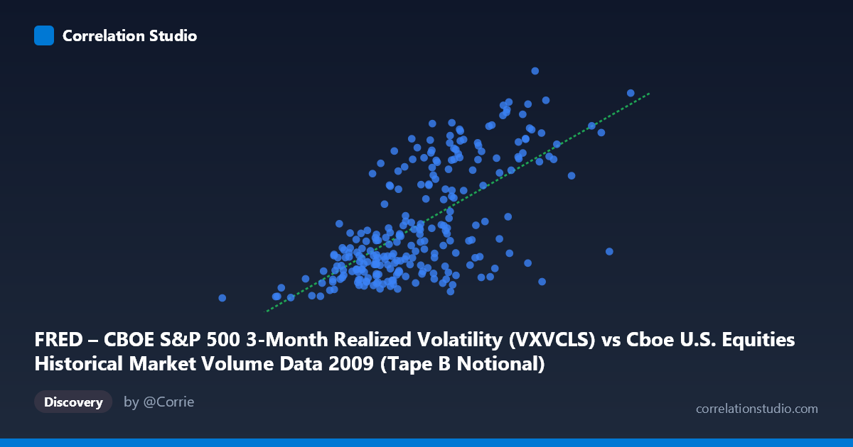
FRED – CBOE S&P 500 3-Month Realized Volatility (VXVCLS) vs Cboe U.S. Equities Historical Market Volume Data 2009 (Tape B Notional)
- Pearson correlation (r)
- 0.6665
- Spearman correlation
- 0.6424
- p-value
- 0
- Sample size (n)
- 252
- 95% confidence interval
- 0.5916 to 0.7299
- Granger causality
- None
- Granger optimal lag
- 1
AI analysis
Analysis: CBOE S&P 500 3-Month Realized Volatility vs. Tape B Notional Volume (2009)
1. Overall Relationship The scatterplot reveals a moderate positive relationship between CBOE S&P 500 3-month realized volatility (X-axis) and Tape B notional trading volume (Y-axis) across U.S. equity exchanges in 2009. As volatility readings rise — spanning roughly 1.3 billion to 9.5 billion in the X range — Tape B notional values tend to climb from the low-20s toward the mid-50s. This pattern is broadly consistent with the well-established market microstructure principle that elevated volatility environments attract greater trading activity, as participants hedge, rebalance, and opportunistically trade around price dislocations. The linear regression equation (y = 4.06E-09x + 11.54) confirms a positive slope, and the visual spread of points generally tracks this upward trend, though with considerable dispersion throughout.
2. Correlation Strength, Statistical Significance, and Causal Direction With r = 0.6665 and r² = 0.4442, the correlation is statistically meaningful but far from deterministic — roughly 44.4% of the variance in Tape B notional volume is explained by realized volatility, leaving over 55% attributable to other forces. The 95% confidence interval of [0.5916, 0.7299] is reassuringly narrow given the sample size of n = 252 drawn from a population of N = 3,232, and the p-value of effectively zero confirms this is not a chance finding. However, the Granger causality results tell a more cautionary story: neither direction (X→Y: F = 0.028, p = 0.868; Y→X: F = 1.18, p = 0.278) reaches significance at conventional thresholds. This means that past values of realized volatility do not reliably predict future Tape B volume, and vice versa — the co-movement captured by the correlation is largely contemporaneous rather than reflecting a temporal lead-lag structure suitable for forecasting.
3. Notable Patterns, Clusters, and Outliers The scatterplot exhibits several distinct features worth highlighting. There is a visible lower-left cluster of points concentrated around X values of 1.3–4.0 billion with Y values in the 22–30 range, likely reflecting calmer market sessions, possibly in the latter half of 2009 as post-crisis volatility began subsiding. A second, more dispersed cluster appears at higher X and Y values (X: 6–9.5 billion; Y: 40–55), representing elevated-volatility sessions with surging notional flows. Notably, the sample points include some apparent outliers or high-leverage observations — for instance, the point near (9.51B, ~47) and (7.07B, 50.43) sit at the upper extreme of both axes and may disproportionately influence the regression slope. There also appears to be heteroscedasticity: variance in Y increases as X increases, suggesting the linear model may underfit the high-volatility regime and that a log-linear or segmented model might better capture the relationship.
4. Confounding Factors and Interpretive Caveats Several important caveats apply. 2009 was an extraordinary year — encompassing the tail of the global financial crisis, the March 2009 market bottom, and a powerful recovery rally — meaning volatility and volume dynamics were regime-dependent in ways unlikely to generalize to normal market years. The axis metadata warrants careful scrutiny: the X-axis is labeled as VXVCLS (a realized volatility measure) but the dataset description references Cboe market volume data, while the Y-axis references Tape B notional but the dataset is described as FRED implied volatility — suggesting a possible axis or dataset labeling inversion that should be verified before drawing firm conclusions. Additionally, Tape B notional volume is influenced by sector composition, ETF activity, and exchange routing decisions that are largely independent of broad volatility indices. Seasonal effects, macroeconomic announcements, and Federal Reserve interventions throughout 2009 could jointly drive both series, creating spurious co-movement.
5. Actionable Insights and Further Investigation Given the moderate but non-causal correlation, practitioners should resist using lagged volatility alone as a volume forecasting signal — the Granger results explicitly caution against this. Instead, further investigation should explore regime-conditional models: separating 2009 into crisis (Q1), trough (Q1–Q2), and recovery (Q2–Q4) sub-periods may reveal that the correlation is substantially stronger in specific regimes. Non-linear modeling (e.g., polynomial regression or spline fits) should be tested given the apparent heteroscedasticity. Analysts should also verify the axis-dataset alignment to ensure interpretations are grounded in correctly mapped variables. Finally, incorporating additional covariates — such as VIX levels, Fed announcement dates, S&P 500 return magnitude, and market breadth indicators — into a multivariate framework would likely improve explanatory power well beyond the 44.4% achieved here and reveal whether the volatility-volume link is direct or merely a proxy for broader market stress.
X dataset: Cboe U.S. Equities Historical Market Volume Data 2009
Y dataset: FRED – CBOE S&P 500 3-Month Realized Volatility
Part of experiment: Daily - Cboe U.S. Equities Historical Market Volume Data 2009 vs FRED – CBOE S&P 500 3-Month Realized Volatility