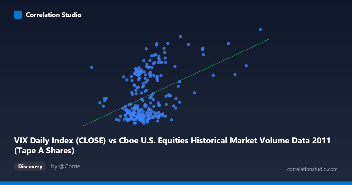
VIX Daily Index (CLOSE) vs Cboe U.S. Equities Historical Market Volume Data 2011 (Tape A Shares)

Pearson correlation (r): 0.4187
Spearman correlation: 0.3334
p-value: 0
Sample size (n): 252
95% confidence interval: 0.3113 to 0.5156
Granger causality: None
Granger optimal lag: 1

AI analysis

Scatterplot Analysis: VIX vs. U.S. Equity Market Volume (2011)

Overall Relationship The scatterplot reveals a moderate positive relationship between U.S. equity market trading volume (X-axis) and the VIX Daily Index close (Y-axis) across 252 trading observations spanning 2011. As market volume increases, VIX levels tend to rise, which is intuitive: heightened volatility typically coincides with heavier trading activity as investors react to uncertainty by buying and selling more aggressively. The linear regression equation (y = 5.07×10⁻⁸x + 9.50) confirms this upward slope, though the scatter around the regression line is visibly substantial, immediately signaling that the relationship is far from deterministic.

Correlation Strength and Statistical Significance The Pearson correlation of r = 0.42 indicates a moderate positive association, but the more telling figure is r² = 0.175, meaning that variation in trading volume explains only 17.5% of the variance in VIX levels. The remaining 82.5% is driven by factors entirely outside this model. The 95% confidence interval for r ([0.311, 0.516]) is meaningfully bounded away from zero, and the p-value of 4.04×10⁻¹² confirms the relationship is highly statistically significant — not a sampling artifact. However, statistical significance here is partly a function of the large population context (N = 3,780), so practical significance should be interpreted cautiously. Critically, Granger causality tests reveal no significant predictive direction in either direction (X→Y: F = 0.07, p = 0.79; Y→X: F = 0.001, p = 0.97), meaning that past values of volume do not help predict future VIX, and vice versa, at a one-period lag. This suggests the correlation reflects contemporaneous co-movement rather than a lead-lag causal mechanism.

Notable Patterns and Outliers Several structural features stand out in the data. There appear to be two loose clusters: a lower-volume, lower-VIX grouping concentrated roughly between 200–350M shares and VIX values of 15–22, and a more dispersed high-VIX cluster at similar or elevated volumes where VIX spikes above 30–40. Sample points like (474.7M, 39.0), (322.9M, 43.0), and (338.9M, 36.3) represent clear high-volatility outliers where VIX is disproportionately elevated relative to volume, likely corresponding to acute stress episodes in mid-to-late 2011 (e.g., the U.S. debt ceiling crisis and European sovereign debt contagion in August–October 2011). Conversely, several high-volume points — such as (367.2M, 24.4) and (361.7M, 24.8) — show only moderate VIX levels, indicating that elevated volume does not always coincide with elevated fear. This asymmetry hints at a non-linear or threshold relationship that a simple linear model may underfit.

Confounding Factors and Caveats Several important caveats apply. First, 2011 was an unusually volatile year dominated by discrete macro shock events, so the VIX spikes visible in the data may be episodic rather than reflective of a stable structural relationship — this limits generalizability to other periods. Second, trading volume itself is influenced by structural market factors (e.g., algorithmic trading, index rebalancing, options expiration days) that have no direct connection to investor fear sentiment captured by VIX. Third, the axes appear to be swapped from convention: VIX is plotted on the Y-axis while volume is on X, but the dataset labels suggest the column assignments may be inverted between datasets, warranting verification of data alignment. Fourth, daily granularity means intraday timing differences between when volume is recorded and when VIX closes could introduce measurement noise. Finally, the lack of Granger causality at lag-1 does not rule out relationships at longer lags or under regime-switching conditions.

Actionable Insights and Further Investigation The moderate but unexplained majority of variance (82.5%) and the absence of Granger causality suggest several productive next steps. Researchers should test non-linear models (e.g., polynomial regression or quantile regression) to capture the apparent threshold behavior at high-VIX episodes. Investigating longer Granger causality lags (e.g., 5–10 days) could reveal delayed feedback loops not visible at lag-1. It would also be valuable to segment the data by market regime — pre- and post-August 2011 shock — to test whether the correlation structure changes materially during stress periods. Adding control variables such as options volume, put/call ratios, or macroeconomic news indicators could substantially improve explanatory power. Finally, replicating this analysis across multiple years would test whether the r = 0.42 finding is robust or a 2011-specific artifact of extreme market conditions.

X dataset: Cboe U.S. Equities Historical Market Volume Data 2011

Y dataset: VIX Daily Index

Part of experiment: Daily - Cboe U.S. Equities Historical Market Volume Data 2011 vs VIX Daily Index