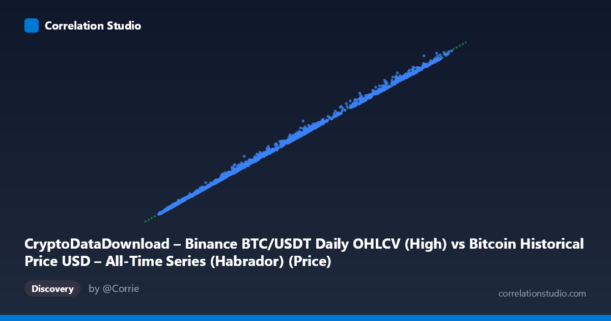
CryptoDataDownload – Binance BTC/USDT Daily OHLCV (High) vs Bitcoin Historical Price USD – All-Time Series (Habrador) (Price)
- Pearson correlation (r)
- 0.9996
- Spearman correlation
- 0.9996
- p-value
- 0
- Sample size (n)
- 3169
- 95% confidence interval
- 0.9996 to 0.9997
- Granger causality
- None
- Granger optimal lag
- 10
- Time coverage
- 2017-08-17 to 2026-04-28
AI analysis
Analysis: BTC/USDT Daily High vs. Bitcoin Historical Price (Habrador)
1. What the Visualization Reveals
This scatterplot compares two ostensibly independent sources reporting on the same underlying phenomenon: Bitcoin's daily price. The near-perfect linear alignment (points hugging a line with slope ≈1.015 and intercept ≈204) indicates these are not two distinct economic variables but two measurements of the same asset price, likely differing only in exchange source (Binance BTC/USDT) or minor methodological details (e.g., "High" vs. a blended price field). The data spans from ~$3,178 to ~$124,720, covering multiple full bull/bear cycles from 2017 through 2026.
2. Strength, Direction, and Statistical Meaning
The correlation is essentially maximal: r = 0.9996, r² = 0.9993, meaning 99.93% of the variance in Y is explained by X — almost no unexplained variation remains. The 95% CI [0.9996, 0.9997] is razor-tight, and p = 0 confirms this relationship is not due to chance at any conventional threshold. However, this level of correlation is far beyond what's typical for genuinely distinct financial variables (e.g., macro indicators, sentiment, volume) — it's the signature of two records of the same quantity, not two variables in a causal or economic relationship. Consequently, the Granger causality result (no significant predictive direction in either direction, p ≈ 0.33 both ways) makes sense: neither series "leads" the other because they're contemporaneous reports of identical price action, not sequentially-related processes. There is no meaningful lead-lag structure to exploit.
3. Notable Patterns and Deviations
The slope of 1.015 (not exactly 1.0) and small positive intercept suggest a slight systematic offset — X-axis values run marginally lower than Y-axis values on average, consistent with X being a "High" price (perhaps daily high from one source) while Y may reflect a different daily reference point (e.g., close, or high from a different exchange/feed) that runs slightly higher, especially during volatile spikes. Since both stdevs are nearly identical (~32,400 vs ~32,900) and increase together, heteroscedasticity is expected but proportional (variance scales with price level, typical of financial data in dollar terms — log-transformed analysis might be more appropriate for price data across orders of magnitude). No visible clusters, regime breaks, or outlier pairs are evident from the sample; deviations from the 1:1 line likely stem from timing/rounding differences rather than structural breaks.
4. Confounding Factors and Caveats
The primary caveat: this is likely a data-integrity check, not a discovery of an economic relationship. Both series describe BTC price from overlapping exchanges/time periods, so the near-unity correlation is mechanically guaranteed rather than informative about market behavior. Confounds to consider: (a) differing snapshot times (daily "High" can differ by exchange/timezone), (b) currency pair nuances (USDT vs. USD may introduce basis/peg deviations), (c) potential lag/misalignment in timestamp joins inflating or slightly denting r, and (d) the Granger test's "10-period optimal lag" is not meaningful here given the data are same-day/contemporaneous — Granger causality is designed for genuinely distinct time series, not duplicate/near-duplicate records.
5. Actionable Insights
- Reframe the analysis goal: rather than treating this as "correlation between two variables," use it as a reconciliation/validation exercise between two BTC price feeds — investigate the intercept (~$204) and slope deviation (1.015) to quantify systematic bias between sources. - Investigate outlier residuals: isolate points with the largest deviation from y = 1.015x + 204 (visually, look for points off the diagonal) — these likely correspond to exchange-specific volatility spikes, flash crashes, or data feed errors and are worth auditing individually. - Log-transform for modeling: given the multi-order-of-magnitude price range (~$3K to ~$125K), a log-log regression would better characterize proportional relationship and heteroscedasticity than raw linear regression. - Drop Granger causality framing: it's not the right tool for two contemporaneous price reports; consider it only if you can establish true temporal offset (e.g., one series reported before the other intraday).
X dataset: Bitcoin Historical Price USD – All-Time Series (Habrador)
Y dataset: CryptoDataDownload – Binance BTC/USDT Daily OHLCV
Part of experiment: Bitcoin - Bitcoin Historical Price USD – All-Time Series (Habrador) vs CryptoDataDownload – Binance BTC/USDT Daily OHLCV