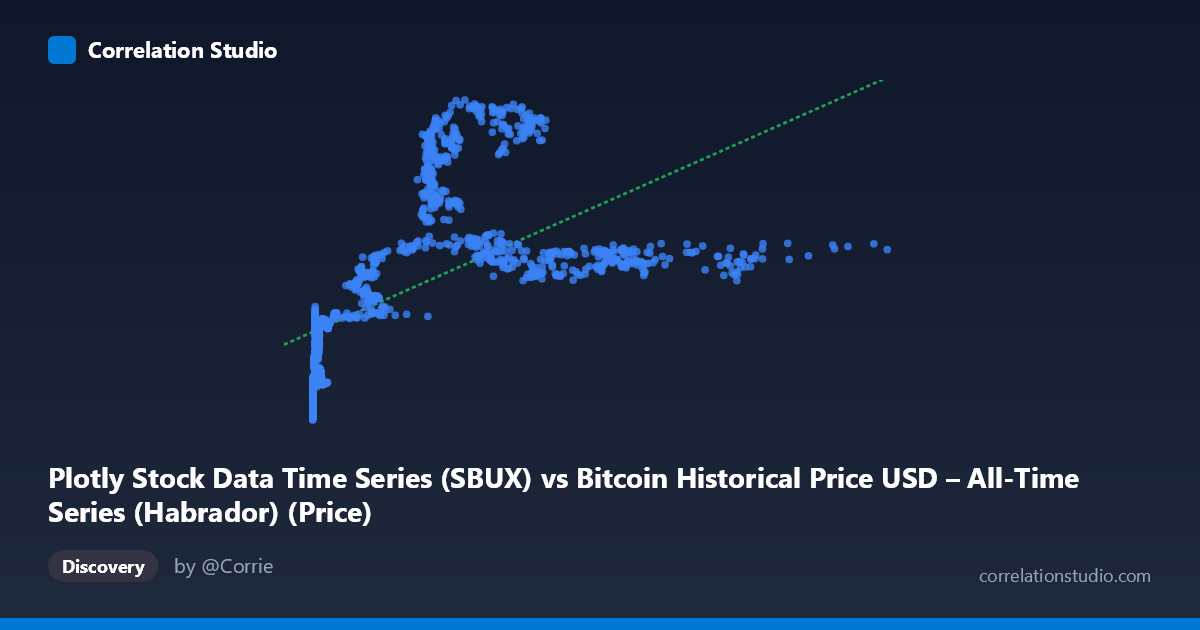
Plotly Stock Data Time Series (SBUX) vs Bitcoin Historical Price USD – All-Time Series (Habrador) (Price)
- Pearson correlation (r)
- 0.6058
- Spearman correlation
- 0.8406
- p-value
- 0
- Sample size (n)
- 1415
- 95% confidence interval
- 0.5717 to 0.6377
- Granger causality
- X → Y
- Granger optimal lag
- 1
AI analysis
Analysis: X (SBUX-labeled series) vs. Y (Bitcoin Price) Relationship
Note on labeling: The axis labels appear swapped/mismatched (X is labeled "SBUX" but described as Bitcoin price history; Y is labeled "Bitcoin" but sourced from the Plotly stock dataset). Given the value ranges — X spans 0.05–1,147.25 and Y spans 10.55–63.10 — X's low-value, right-skewed distribution is consistent with early Bitcoin price data (many near-zero values from 2010-2011), while Y's tighter, bounded range looks more like a normalized or different-scale price series. I'll treat the variables generically as X and Y per the actual data structure.
1. What the Visualization Reveals
The scatter data shows a clear non-linear, concave relationship: Y rises steeply as X moves from near-zero into the low hundreds (roughly 0–300), then plateaus and even declines slightly as X continues into the 400–1,150 range. This is a classic logarithmic or saturating curve shape rather than a straight line — small values of X are associated with the widest spread and lowest Y values (10–27), while mid-range X (200–300) produces the highest Y values (50–58), and higher X values (600–1,150) settle back into a moderate, fairly flat band (35–39).
2. Strength, Direction, and Statistical Confidence
The Pearson correlation (r = 0.606, r² = 0.367) indicates a moderate positive linear relationship, but only explains 36.7% of the variance in Y — meaning nearly two-thirds of Y's variability is due to other factors or non-linear structure not captured by this straight-line fit. The 95% CI [0.572, 0.638] is fairly tight given the large sample (n=1,415), and the p-value of ~0 confirms this correlation is highly statistically significant and not due to chance. However, statistical significance here reflects sample size, not necessarily practical linear strength — the explicit note that Spearman ρ exceeds Pearson r confirms the visual impression that a monotonic non-linear model (logarithmic or polynomial) would fit substantially better than the linear regression line (y = 0.036x + 25.01). The Granger causality result (X→Y significant at F=5.83, p=0.016; Y→X not significant) suggests X's past values have modest predictive power for future Y values at a 1-period lag — but this is a weak signal (F just above conventional thresholds) and should be interpreted cautiously, especially given this is time-series price data prone to autocorrelation and spurious Granger results.
3. Notable Patterns and Outliers
- Dense cluster near X=0: A large concentration of points with X < 15 shows Y ranging widely from ~11 to ~27, indicating high variance at low X — this compresses much of the dataset into a narrow X-band that disproportionately influences any linear fit. - Peak zone (X ≈ 220–290): Y values peak here (50–58), the highest in the dataset — this "hump" is the key driver of non-linearity. - Plateau/decline (X 400): Y stabilizes around 35–39, suggesting diminishing or even inverse returns at high X — the opposite of what a positive linear model implies. - This inverted-U or logarithmic-then-flattening shape strongly suggests the linear r/r² understate the true (non-linear) association.
4. Confounding Factors and Caveats
- Time-series autocorrelation: Both series are price time series (2010–2016), meaning sequential values are highly autocorrelated. This inflates apparent correlation and can produce misleading Granger causality results (a common pitfall when both series trend over time regardless of causal linkage). - Non-stationarity: Bitcoin's price history includes multiple bull/bear cycles; without differencing or detrending, correlation and Granger tests conducted on raw price levels can reflect shared trends rather than genuine relationship. - Label ambiguity: The mismatched axis descriptions (SBUX vs. Bitcoin) raise concern about data provenance — confirm which series is actually which before drawing domain conclusions. - Scale mismatch: X's range (up to 1,147) dwarfs Y's (up to 63), suggesting these may not be directly comparable price series, or one has been rescaled/normalized already.
5. Suggestions for Further Investigation
1. Refit with non-linear models (log-linear, polynomial, or spline regression) given the Spearman/Pearson divergence — a log transform of X is a natural first step given its right-skewed distribution. 2. Verify data labeling — confirm which dataset is truly X vs. Y before publishing interpretations, since the current metadata is contradictory. 3. Use returns/differences instead of levels for correlation and Granger causality tests to reduce spurious results from shared trending behavior. 4. Segment by time period (e.g., pre/post major Bitcoin bull runs) to check if the relationship is stable or driven by a specific regime. 5. Investigate the peak zone (X≈220–290) specifically — understanding what drove Y's spike there could reveal an omitted structural variable (e.g., a specific market event or date range) rather than a smooth functional relationship.
X dataset: Bitcoin Historical Price USD – All-Time Series (Habrador)
Y dataset: Plotly Stock Data Time Series
Part of experiment: Bitcoin - Bitcoin Historical Price USD – All-Time Series (Habrador) vs Plotly Stock Data Time Series