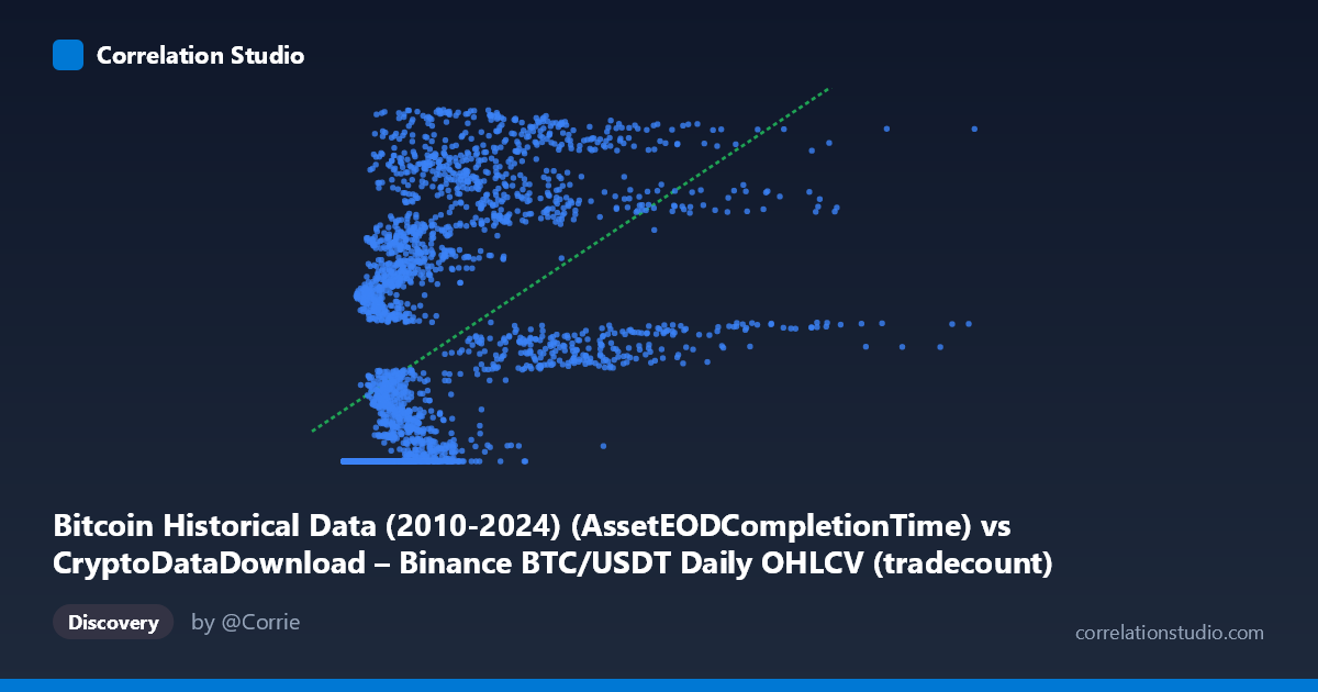
Bitcoin Historical Data (2010-2024) (AssetEODCompletionTime) vs CryptoDataDownload – Binance BTC/USDT Daily OHLCV (tradecount)
- Pearson correlation (r)
- 0.5264
- Spearman correlation
- 0.7892
- p-value
- 0
- Sample size (n)
- 3191
- 95% confidence interval
- 0.5009 to 0.5511
- Granger causality
- None
- Granger optimal lag
- 10
- Time coverage
- 2017-08-17 to 2026-05-20
AI analysis
Analysis: Bitcoin Timestamp vs. Trade Count Relationship
1. What the Visualization Reveals
This scatterplot is somewhat unusual in that the X-axis ("AssetEODCompletionTime") appears to be a timestamp-like value rather than a conventional price or volume metric, plotted against Y (tradecount). The data shows a distinctive step-like or threshold pattern: a large cluster of points sits at a floor value near Y≈1,614,337,000 across a wide range of X values (roughly 0 to ~2 million), followed by a steep upward climb where Y rises sharply (up to ~1,779,000,000) as X increases further. This is not a smooth linear cloud but rather resembles two regimes — a flat baseline segment and a rapidly ascending segment — consistent with the note that Spearman's ρ exceeds Pearson's r, confirming non-linear structure.
2. Strength, Direction, and Uncertainty
The Pearson correlation (r = 0.526) indicates a moderate positive relationship, with R² = 0.277 meaning only 27.7% of the variance in Y is explained by X — the majority (72%) remains unexplained by this linear model. The 95% CI [0.501, 0.551] is fairly tight given the large sample (n=3,191), and the p-value of ~0 confirms this correlation is statistically robust and not due to chance. However, statistical significance here reflects sample size more than practical predictive strength — a moderate r with a large N is common and doesn't imply Y can be reliably forecast from X. Critically, the Granger causality tests show no significant predictive direction in either direction (X→Y: p=0.447; Y→X: p=0.657), meaning that despite the contemporaneous correlation, neither variable helps forecast future values of the other in a time-series sense. This suggests the relationship, while real, is likely driven by a shared trend or structural break rather than genuine causal/temporal linkage.
3. Notable Patterns and Outliers
The clearest feature is the flat "floor" cluster: many points (e.g., X < 1,000,000) sit at nearly identical Y-values (~1,614,337,xxx), suggesting a data artifact — possibly a placeholder, minimum threshold, or period of missing/interpolated tradecount data early in the series. This is followed by a transition zone (roughly X = 1M–5M) where Y rapidly increases and becomes more variable, and a sparser high-X tail (X 5M) with elevated, more scattered Y-values up to ~1.78 billion. This pattern strongly resembles a time-series regime shift rather than a continuous functional relationship — consistent with X potentially encoding elapsed time or a cumulative/sequential index rather than an independent price variable.
4. Confounding Factors and Caveats
Several caveats are important: - Variable identity ambiguity: X is labeled as an "AssetEODCompletionTime" (a timestamp), not a typical price/volume field — this makes a Pearson correlation with tradecount conceptually unusual and likely reflects a shared time trend (both variables increasing over the 2017–2026 period) rather than a direct economic relationship. - Autocorrelation: Both series are time-ordered and likely non-stationary (trending), which inflates correlation coefficients independent of any real link — classic spurious correlation risk. - The flat baseline segment suggests data quality issues (e.g., default/fill values) in early records that could be distorting the correlation estimate. - Non-linearity: Since Spearman ρ Pearson r, a monotonic but non-linear (e.g., logarithmic, sigmoid, or piecewise) relationship is more appropriate than the linear model presented.
5. Actionable Insights
1. Clarify variable definitions — confirm whether X truly represents a timestamp; if so, this analysis is essentially examining tradecount's growth over time, and a proper time-series model (with trend/seasonality decomposition) is more appropriate than cross-sectional correlation. 2. Investigate the flat-floor cluster for potential data quality issues (missing values imputed with a constant). 3. Re-run correlation after detrending both series (e.g., first differences) to test for genuine relationship beyond shared trend — this would also make the Granger causality test more reliable, since Granger tests assume stationarity. 4. Fit non-linear models (piecewise regression, logistic/log curves) given the R² gap between Pearson and Spearman metrics. 5. Given the lack of Granger causality, do not use this pair for predictive forecasting; treat the correlation as descriptive/structural rather than causal or forecastable.
X dataset: CryptoDataDownload – Binance BTC/USDT Daily OHLCV
Y dataset: Bitcoin Historical Data (2010-2024)
Part of experiment: Bitcoin - CryptoDataDownload – Binance BTC/USDT Daily OHLCV vs Bitcoin Historical Data (2010-2024)