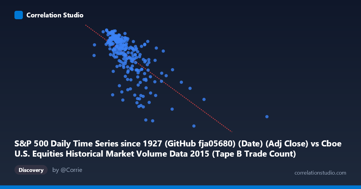
S&P 500 Daily Time Series since 1927 (GitHub fja05680) (Date) (Adj Close) vs Cboe U.S. Equities Historical Market Volume Data 2015 (Tape B Trade Count)

Pearson correlation (r): -0.6663
Spearman correlation: -0.7066
p-value: 0
Sample size (n): 252
95% confidence interval: -0.7298 to -0.5914
Granger causality: None
Granger optimal lag: 1

AI analysis

Analysis: S&P 500 Adjusted Close vs. Cboe Tape B Trade Count (2015)

Relationship Overview The scatterplot reveals a moderately strong negative relationship between the S&P 500 adjusted closing price (X-axis) and Cboe Tape B trade counts (Y-axis) across 252 trading days in 2015. As the S&P 500 price level increases, Tape B trade counts tend to decrease, and vice versa. The linear regression equation (y = −0.000392x + 2178.46) confirms this inverse slope, meaning that for every 100,000-unit increase in the S&P 500 price index value, Tape B trade count decreases by approximately 39 units. The relationship is visually apparent as a downward-sloping cloud of points, though with considerable scatter around the regression line.

Correlation Strength and Statistical Significance The Pearson correlation of r = −0.6663 indicates a moderate-to-strong negative association, and the R² of 0.4439 means that approximately 44.4% of the variance in Tape B trade counts is explained by the S&P 500 price level — a meaningful but incomplete explanatory relationship, leaving over 55% of variance attributable to other factors. The 95% confidence interval of [−0.7298, −0.5914] is relatively narrow and entirely negative, reinforcing confidence that the inverse relationship is genuine and not a statistical artifact. With a p-value effectively at zero across a paired sample of n = 252 (drawn from a population of N = 3,302), the result is highly statistically significant. However, the Granger causality tests yield no significant directional predictive relationship in either direction (X→Y: F = 0.245, p = 0.621; Y→X: F = 0.042, p = 0.839), meaning that knowing today's S&P 500 price does not meaningfully improve predictions of tomorrow's Tape B trade count at a one-period lag, and vice versa. This critical finding decouples statistical correlation from temporal predictive utility.

Notable Patterns, Clusters, and Outliers Several structural features stand out in the data. The bulk of observations cluster between S&P 500 values of roughly 200,000–400,000 (on the adjusted close scale used here) and Tape B trade counts between approximately 2,000–2,130, forming a dense core with a visible downward trend. However, there is a notable right-tail extension with a sparse cluster of extreme X-values reaching up to ~1,014,000 — far beyond the main distribution — associated with markedly lower trade counts (approaching 1,867–1,970). Points such as (640,679, 1,867.61) and (621,009, 1,970.89) appear as potential outliers or high-leverage observations that may disproportionately influence the regression slope. Within the main cluster, vertical dispersion is substantial, suggesting considerable day-to-day variability in trade counts at similar price levels. There is also a possible non-linear or threshold pattern: the relationship appears steeper at higher X-values, hinting that a logarithmic or piecewise model might better capture the true functional form.

Confounding Factors and Interpretive Caveats Several important caveats apply. First, the X-axis label suggests a dataset join artifact — the "S&P 500 Adjusted Close" appears to be serving as a date-aligned index rather than a conventional price in the hundreds or thousands, with values ranging from 130,085 to over 1,000,000, which is inconsistent with typical S&P 500 levels in 2015 (~1,900–2,130). This strongly suggests either a data scaling issue, a cumulative or transformed metric, or a misalignment in the dataset merge, which would fundamentally alter the economic interpretation. Second, both variables may be jointly driven by market volatility regimes: high-volatility periods (e.g., the August 2015 correction) would simultaneously depress equity prices and alter trading volumes across venues, creating a spurious or context-dependent correlation. Third, Tape B specifically covers NYSE American and regional exchange listings — changes in exchange market share, ETF trading patterns, or regulatory events in 2015 could independently shift trade counts without direct causation from the S&P 500 level.

Actionable Insights and Further Investigation Given the Granger non-causality result, practitioners should not use S&P 500 price levels as a predictive signal for Tape B trade counts in short-term trading or market-microstructure models. However, the 44% shared variance warrants deeper investigation. Recommended next steps include: (1) auditing the X-axis data transformation to confirm whether the values represent true adjusted closing prices or a derived metric, as this is critical to any economic interpretation; (2) testing whether VIX or realized volatility acts as a common driver explaining the correlation, by including it as a control variable in a multivariate regression; (3) fitting a log-linear or segmented regression model to assess whether the apparent non-linearity at high X-values reflects a genuine regime change or outlier influence; and (4) extending the Granger causality test to longer lags (2–5 periods) to rule out delayed predictive relationships. Decomposing the data by market regime (pre- vs. post-August 2015 correction) could also reveal whether the correlation is stable or episodic.

X dataset: Cboe U.S. Equities Historical Market Volume Data 2015

Y dataset: S&P 500 Daily Time Series since 1927 (GitHub fja05680) (Date)

Part of experiment: Daily - Cboe U.S. Equities Historical Market Volume Data 2015 vs S&P 500 Daily Time Series since 1927 (GitHub fja05680) (Date)