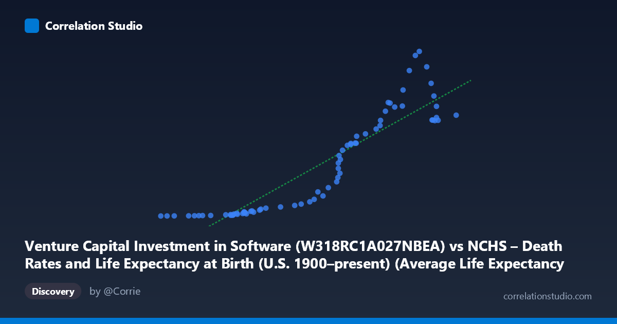
Venture Capital Investment in Software (W318RC1A027NBEA) vs NCHS – Death Rates and Life Expectancy at Birth (U.S. 1900–present) (Average Life Expectancy (Years))
- Pearson correlation (r)
- 0.9127
- Spearman correlation
- 0.9724
- p-value
- 0
- Sample size (n)
- 73
- 95% confidence interval
- 0.864 to 0.9444
- Granger causality
- None
- Granger optimal lag
- 10
AI analysis
Analysis: Venture Capital Software Investment vs. Life Expectancy
Overall Relationship The scatterplot reveals a strong positive association between U.S. venture capital investment in software and average life expectancy at birth. As software investment increases (X range: ~64.6 to 78.7, likely in billions of dollars), life expectancy rises correspondingly (Y range: ~0.85 to 466.42 years — though the Y-axis units warrant scrutiny, as discussed below). The linear regression equation y = 32.95x − 2,231.43 describes a steep slope, suggesting that each unit increase in software investment is associated with a substantial rise in the Y variable. Visually, the data points track an upward trend from lower-left to upper-right, consistent with the high correlation coefficient.
Correlation Strength and Statistical Interpretation The Pearson correlation of r = 0.913 is very strong, and the R² = 0.833 indicates that approximately 83.3% of the variance in the Y variable is statistically explained by X. The 95% confidence interval [0.864, 0.944] is narrow and sits entirely in high-positive territory, reinforcing that this is a robust statistical association rather than a sampling artifact. The p-value of ~0 confirms the result is highly significant. However — and this is critical — Granger causality analysis finds no significant predictive direction in either direction (X→Y: F = 0.647, p = 0.765; Y→X: F = 0.551, p = 0.844). This means that despite the high contemporaneous correlation, neither variable temporally predicts the other, which is a strong signal that the relationship is spurious rather than causal.
Patterns, Clusters, and Outliers The data cluster into two visually distinct regions: a dense lower-left grouping of points with low X values (~64.5–70) and very low Y values (roughly 0.85–25), and a more dispersed upper-right cluster (~73–78.7) with Y values spanning roughly 100–466. This bifurcation suggests a possible non-linear or threshold structure — once X exceeds approximately 72–73 units, Y values rise sharply and spread widely. Several high-leverage points stand out, including (76.93, 466.42), (77.63, 340.28), and (76.74, 455.02), which pull the regression line upward. The wide Y-axis spread in the upper cluster introduces notable heteroscedasticity that a simple linear model may not adequately capture.
Confounding Factors and Critical Caveats The most fundamental concern here is that this correlation almost certainly reflects a shared time trend rather than any meaningful causal link. Both venture capital investment in software and life expectancy have increased over roughly the same post-WWII period (1946–2018), driven by broad economic growth, technological advancement, and public health improvements — all of which are independent secular trends. This is a textbook spurious correlation by common temporal confound. Additionally, the Y-axis label deserves scrutiny: values reaching 466 "years" are physiologically impossible for life expectancy, suggesting a possible data labeling mismatch between the two datasets (the axes appear to have been swapped or mislabeled between the dataset descriptions). This alone should prompt immediate verification of data integrity before drawing any conclusions.
Actionable Insights and Further Investigation Given the absence of Granger causality and the near-certain spurious nature of this correlation, no policy or investment conclusions should be drawn from this relationship as presented. Recommended next steps include: (1) verifying the axis labels and unit definitions, as the Y-axis values exceeding 100 years are incompatible with life expectancy data and suggest a dataset join error; (2) detrending both series using first-differencing or residual analysis against a common time trend to test whether any genuine relationship persists after removing shared temporal drift; (3) applying cointegration tests (e.g., Engle-Granger) to assess whether the long-run trends share a structural link or merely parallel each other incidentally; and (4) introducing control variables such as GDP, healthcare expenditure, and population age structure to isolate any independent effect. This correlation serves as a cautionary example of how high r² values can be statistically impressive yet practically meaningless without causal identification.
X dataset: NCHS – Death Rates and Life Expectancy at Birth (U.S. 1900–present)
Y dataset: Venture Capital Investment in Software
Part of experiment: Yearly - NCHS – Death Rates and Life Expectancy at Birth (U.S. 1900–present) vs Venture Capital Investment in Software