NOAA ISD Weather Station History (Lat/Lon Index) (SLP_ATTRIBUTES) vs CryptoDataDownload – Binance BTC/USDT Daily OHLCV (Open)
- Pearson correlation (r)
- -0.4704
- Spearman correlation
- -0.3123
- p-value
- 0
- Sample size (n)
- 355
- 95% confidence interval
- -0.5476 to -0.3851
- Granger causality
- None
- Granger optimal lag
- 1
- Time coverage
- 2024-01-01 to 2024-12-31
AI analysis
Analysis of the Scatterplot Relationship
1. What the visualization reveals
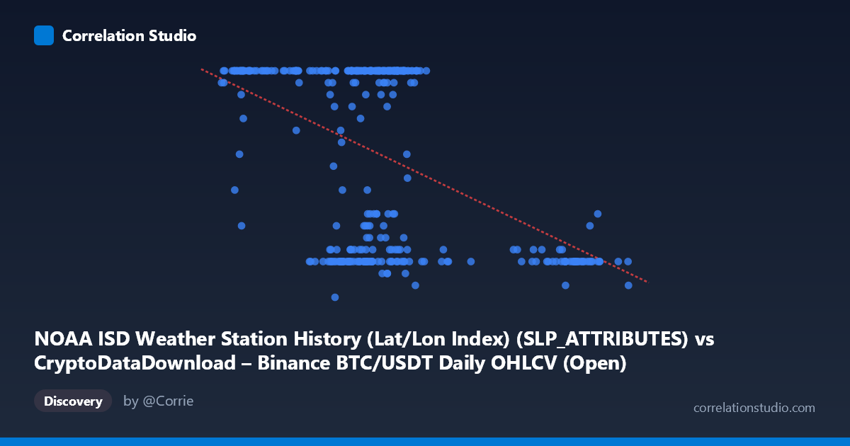
The scatterplot shows a moderate negative relationship between the X variable (labeled as a weather station attribute field but populated with what appear to be BTC/USDT price-like values) and Y (ranging 5–24, likely a bounded/categorical-feeling variable despite being treated as continuous). The data is heavily clustered in the X range of ~60,000–70,000, with a secondary cluster near 95,000–100,000 that shows consistently low Y values (7–11). This bimodal clustering in X, combined with the compressed integer-like values in Y, suggests the underlying data may not be a simple continuous bivariate relationship but rather two overlapping regimes or populations.
2. Strength, direction, and statistical confidence
The correlation coefficient (r = -0.470) indicates a moderate negative linear relationship: as X increases, Y tends to decrease. However, r² = 0.221 tells us that only about 22% of the variance in Y is explained by X — the remaining ~78% is driven by other factors, noise, or non-linear structure not captured by this simple linear model. The 95% CI [-0.548, -0.385] is reasonably tight and excludes zero, and the p-value of ~0 confirms the correlation is statistically significant and not due to chance at this sample size (n=355). That said, statistical significance with a large n does not imply practical strength — the effect is real but modest, explaining roughly one-fifth of the variability. Critically, the Granger causality tests show no significant predictive direction in either direction (X→Y: p=0.71; Y→X: p=0.26), meaning neither variable helps forecast the other over time. This strongly suggests the correlation is contemporaneous/structural rather than causal or lagged-predictive.
3. Notable patterns and outliers
The data reveals at least two distinct clusters: a dense cluster around X≈60,000–70,000 where Y spans the full range (7 to 24) somewhat erratically, and a sparser cluster around X≈90,000–100,000 where Y is consistently low (7–11). This pattern looks less like a smooth linear trend and more like two sub-populations with different means — the high-X cluster pulls the regression line downward, partially manufacturing the appearance of a linear negative correlation. Within the main cluster, Y values cluster heavily at 24 (a ceiling) and at 8–12 (a floor), with fewer intermediate values — hinting that Y may behave more like a discrete or bounded/capped metric rather than a smooth continuous variable.
4. Confounding factors and caveats
The metadata is a significant red flag: axis labels appear mismatched/swapped (X is labeled a NOAA weather attribute column but contextually resembles cryptocurrency price data; Y is labeled a crypto "Open" price but ranges only 5–24, more consistent with a weather/time-based index or count). This mismatch strongly suggests a data-pipeline or column-mapping error, meaning the "relationship" being measured may not reflect what the labels claim. Additionally, combining two unrelated datasets (crypto OHLCV and weather station records) via merge/join on date or index can produce spurious correlations with no causal meaning — a classic case of confounding via a shared join key (e.g., calendar date) rather than genuine covariation. The clustering pattern also suggests a lurking categorical variable (e.g., season, station ID, or market regime) driving both X and Y independently.
5. Recommendations for further investigation
Before drawing conclusions, verify the axis/column mapping — confirm which raw fields were actually plotted, as the current labels appear internally inconsistent. Next, investigate the two apparent X-clusters separately (e.g., segment analysis or a mixture model) to determine whether the overall negative correlation is an artifact of cluster means rather than a true within-group trend. Consider treating Y as ordinal/discrete given its narrow integer range and reduced cardinality, and apply Spearman rank correlation to check robustness to non-linearity. Finally, since Granger causality shows no temporal lead-lag relationship, any predictive modeling effort should treat X and Y as independently evolving series rather than assume one drives the other — further exploration should focus on identifying the true confound (e.g., date, station location, or market/weather regime) linking the two datasets.
X dataset: CryptoDataDownload – Binance BTC/USDT Daily OHLCV
Y dataset: NOAA ISD Weather Station History (Lat/Lon Index)
Part of experiment: Bitcoin - CryptoDataDownload – Binance BTC/USDT Daily OHLCV vs NOAA ISD Weather Station History (Lat/Lon Index)