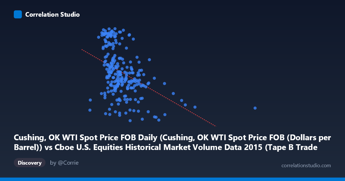
Cushing, OK WTI Spot Price FOB Daily (Cushing, OK WTI Spot Price FOB (Dollars per Barrel)) vs Cboe U.S. Equities Historical Market Volume Data 2015 (Tape B Trade Count)
- Pearson correlation (r)
- -0.4269
- Spearman correlation
- -0.4443
- p-value
- 0
- Sample size (n)
- 252
- 95% confidence interval
- -0.5229 to -0.3202
- Granger causality
- None
- Granger optimal lag
- 1
AI analysis
Analysis: WTI Crude Oil Spot Price vs. Cboe Tape B Trade Count (2015)
Relationship Overview The scatterplot reveals a moderate negative relationship between WTI crude oil spot prices (X-axis, in dollars per barrel) and Cboe Tape B trade counts (Y-axis). As oil prices increase, trade counts tend to decline, and this pattern is visible as a downward-sloping cloud of points. The linear regression equation (y = −3.12×10⁻⁵x + 58.01) confirms this inverse direction, though the scatter around the regression line is substantial. This relationship is intuitive in a broad sense: 2015 was a year of significant oil price decline, and periods of lower oil prices may coincide with heightened market activity and volatility-driven trading in smaller-cap or regional exchange-listed securities captured by Tape B.
Correlation Strength and Statistical Significance The Pearson correlation of r = −0.427 indicates a moderate negative association, but the explained variance tells a more sobering story: r² = 0.182, meaning oil prices account for only 18.2% of the variance in Tape B trade counts. Over 80% of the variation in trading activity is driven by other factors entirely. The 95% confidence interval of [−0.523, −0.320] is meaningfully away from zero, and the p-value of 1.4×10⁻¹² — derived from a population of N = 3,302 daily observations — confirms this correlation is highly statistically significant and unlikely to be a chance artifact. However, statistical significance here is partly a function of the large population size, which demands caution in overinterpreting practical magnitude. Critically, Granger causality tests find no significant predictive direction in either direction (X→Y: F = 0.17, p = 0.68; Y→X: F = 0.64, p = 0.42), meaning that despite the contemporaneous correlation, neither variable meaningfully predicts the other at a one-period lag. This is an important constraint: the relationship reflects co-movement, not a temporal lead-lag dynamic suitable for forecasting.
Notable Patterns, Clusters, and Outliers Several structural features stand out in the data. There appears to be a bimodal or segmented distribution in Y (trade counts), with many observations clustering at higher values (~55–61 barrels) at lower X values and another cluster of moderate-to-low trade counts (~38–50) spread across a wider range of oil prices. A small number of high-X outliers (notably points near 621,009 and 640,679 on the X-axis with relatively low trade counts around 39–40) sit well beyond the main data cloud and likely correspond to anomalous trading volume days or data irregularities. These leverage points could disproportionately influence the regression slope. The bulk of observations concentrate in the X range of roughly 130,000–400,000, where the relationship appears strongest and most consistent.
Confounding Factors and Interpretive Caveats Several important caveats apply. First, 2015 was an unusual year for oil markets, characterized by a sustained price collapse from ~$60 to below $35/barrel, so the correlation may partly reflect a shared time trend rather than a causal mechanism — both variables could be responding independently to macroeconomic conditions (Federal Reserve policy, China growth fears, USD strength). Second, Tape B trade counts capture a specific subset of U.S. equity market activity (NYSE American and regional exchanges), and changes in market structure, exchange competition, or reporting rule changes in 2015 could introduce non-stationarity. Third, the dataset labels appear to be swapped in the axis descriptions (the X-axis dataset is labeled as originating from the Cboe volume file while the Y-axis is labeled from the WTI file), suggesting a possible data joining artifact that warrants verification before drawing firm conclusions.
Actionable Insights and Further Investigation Given the moderate but incomplete correlation and the absence of Granger causality, practitioners should not use oil prices as a standalone predictor of Tape B trading volume. Instead, the following next steps are recommended: (1) Decompose the time series for both variables to separate trend, seasonal, and cyclical components, then re-test correlation on residuals to isolate genuine co-movement from shared trending; (2) Expand the model by incorporating VIX (volatility index), USD/oil currency dynamics, and broad equity market volume as covariates to test whether the oil-trade count link survives multivariate controls; (3) Investigate the high-X outliers explicitly — identifying the specific trading dates could reveal whether they correspond to known market events (e.g., OPEC announcements, earnings seasons) that independently drove both variables; (4) Extend the time window beyond 2015 to test whether this correlation is a regime-specific artifact of the oil bear market or a more persistent structural relationship.
X dataset: Cboe U.S. Equities Historical Market Volume Data 2015
Y dataset: Cushing, OK WTI Spot Price FOB Daily
Part of experiment: Daily - Cboe U.S. Equities Historical Market Volume Data 2015 vs Cushing, OK WTI Spot Price FOB Daily