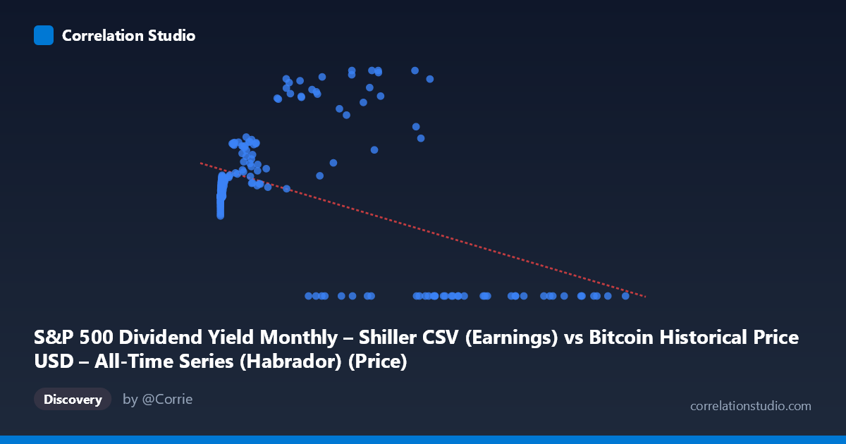
S&P 500 Dividend Yield Monthly – Shiller CSV (Earnings) vs Bitcoin Historical Price USD – All-Time Series (Habrador) (Price)
- Pearson correlation (r)
- -0.4597
- Spearman correlation
- 0.0044
- p-value
- 0
- Sample size (n)
- 189
- 95% confidence interval
- -0.5653 to -0.3392
- Granger causality
- X → Y
- Granger optimal lag
- 4
AI analysis
Analysis: Bitcoin Price vs. S&P 500 Dividend Yield Relationship
1. What the Visualization Reveals
The scatterplot shows a scattered, moderately noisy relationship between the two variables, with a noticeable negative slope but substantial dispersion around it. A large cluster of points sits at low X values (under ~30,000) with Y values concentrated in the 80-140 range, while a distinct subgroup of high-X points (roughly 30,000-120,000) shows a bifurcated pattern: some cluster near Y=0 while others reach the highest Y values in the dataset (160-198). This bifurcation is the most visually striking feature and suggests the relationship is not simply linear.
2. Strength, Direction, and Statistical Confidence
The correlation coefficient (r = -0.4597) indicates a moderate negative relationship, but r² = 0.2113 reveals that only about 21% of the variance in Y is explained by X — meaning roughly 79% of Y's variability stems from other factors entirely. The 95% CI [-0.5653, -0.3392] is reasonably tight and excludes zero, and the p-value (2.85E-11) confirms this correlation is highly statistically significant and not due to chance, given the sample size (n=189 from a population of 1,865). However, statistical significance here reflects reliable detection of a relationship, not necessarily strong practical predictive power — a 21% variance explanation leaves considerable room for unexplained movement. The Granger causality result adds a temporal dimension: X predicts future Y values (F=2.72, p=0.031) at a 4-period lag, while Y does not predict X (p=0.27), suggesting a unidirectional lead-lag relationship where X-axis movements precede changes in Y, rather than mere contemporaneous association.
3. Notable Patterns and Outliers
The most important non-linear feature is the cluster of high-X points with Y=0 exactly — these appear to be either data artifacts, structural breaks, or a regime where the underlying relationship fundamentally changes (e.g., missing/zero-filled data rather than true zero prices). Simultaneously, other high-X points reach the dataset's maximum Y values (~198), creating a "fork" pattern at the high end of X that a single linear fit cannot capture well. At low X values (under 1,000), Y clusters tightly around 85-105, suggesting a compressed, low-variance regime distinct from the high-X behavior. This heteroscedasticity (variance increasing with X) violates a key linear regression assumption.
4. Confounding Factors and Caveats
Given the metadata, this dataset pairing is unusual and likely mismatched: the X-axis is labeled as S&P 500 Dividend Yield while the file/column names reference Bitcoin price data, and vice versa for Y. This labeling confusion (columns cross-referencing the wrong dataset) makes economic interpretation hazardous — it's unclear whether X truly represents dividend yield or Bitcoin price magnitude. Additionally, both Bitcoin prices and financial yields are highly non-stationary time series with trends, volatility clustering, and regime shifts (e.g., BTC's exponential growth phases), which can produce spurious correlations and unreliable Granger causality results if not properly differenced/detrended. The zero-Y cluster strongly suggests a data quality issue (padding, missing values, or misaligned date ranges across the 2010-2026 span) rather than genuine economic signal.
5. Actionable Insights
Before drawing economic conclusions, clarify and correct the column/dataset labeling to ensure X and Y are correctly identified. Investigate the Y=0 cluster specifically — determine if these represent legitimate data points, missing-data placeholders, or a date-range mismatch between the two source series. Given the non-stationarity of both series, rerun the correlation and Granger tests on log-differenced or percentage-change data rather than raw levels, which will reduce spurious correlation risk and better isolate genuine causal signal. Finally, consider segmenting the analysis by X-value regime (low vs. high) or by time period to test whether the relationship is stable or driven by a specific market era (e.g., a particular Bitcoin bull/bear cycle).
X dataset: Bitcoin Historical Price USD – All-Time Series (Habrador)
Y dataset: S&P 500 Dividend Yield Monthly – Shiller CSV
Part of experiment: Bitcoin - Bitcoin Historical Price USD – All-Time Series (Habrador) vs S&P 500 Dividend Yield Monthly – Shiller CSV