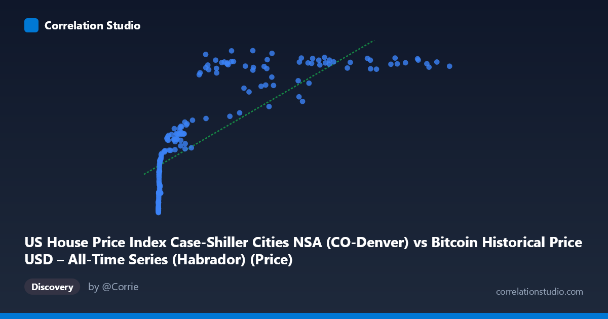
US House Price Index Case-Shiller Cities NSA (CO-Denver) vs Bitcoin Historical Price USD – All-Time Series (Habrador) (Price)
- Pearson correlation (r)
- 0.7925
- Spearman correlation
- 0.9525
- p-value
- 0
- Sample size (n)
- 191
- 95% confidence interval
- 0.733 to 0.84
- Granger causality
- None
- Granger optimal lag
- 9
- Time coverage
- 2010-08-01 to 2026-06-01
- Recomputed on refreshed data
- 2026-10-24 (r was 0.788)
AI analysis
Analysis: Bitcoin Price vs. Case-Shiller Denver Home Price Index
1. What the Visualization Reveals
The scatterplot shows a strong positive association between Bitcoin's historical USD price and the Denver metro Case-Shiller Home Price Index (NSA). At low Bitcoin price levels (under $1,000), the Denver HPI clusters tightly between 120–200, reflecting the pre-2017 era when Bitcoin was a negligible, low-value asset and home prices were rising steadily on their own trajectory. As Bitcoin's price climbs into the tens of thousands, the HPI rises correspondingly into the 280–330 range. The relationship is not linear across the full domain—it looks more like a curve that rises steeply at low X values, then flattens somewhat at higher Bitcoin prices, which is consistent with the note that Spearman's ρ exceeds Pearson's r.
2. Strength, Direction, and Uncertainty
With r = 0.78 and r² = 0.614, roughly 61% of the variance in the Denver HPI is statistically associated with Bitcoin price levels—a strong correlation by conventional standards. The 95% CI [0.72, 0.83] is tight and does not cross zero, and the p-value of ~0 confirms this relationship is highly unlikely to be due to chance in this sample. However, correlation here almost certainly reflects shared time trends rather than a causal economic link. This is strongly reinforced by the Granger causality tests: neither direction (Bitcoin→HPI or HPI→Bitcoin) shows significant predictive power (p = 0.56 and p = 0.80, respectively). In other words, past values of one series do not help forecast future values of the other—the correlation is likely a byproduct of both series trending upward over the same 2010–2026 calendar period rather than genuine interdependence.
3. Notable Patterns and Outliers
The data show a clear log-like or power-law curve rather than a straight line: Bitcoin's price spans over 6 orders of magnitude (0.06 to 118,670) while HPI only ranges from ~120 to 332. Most low-X points compress near Y≈125–160, while mid-to-high Bitcoin prices (10,000–120,000) correspond to a much narrower, higher HPI band (280–330), suggesting diminishing marginal association—large Bitcoin price swings at the high end correspond to much smaller HPI changes. A few points deviate from the general trend, such as (29,111.52, 246.44) and (45,092.81, 259.20), which sit notably below the HPI values of neighboring Bitcoin price levels, likely corresponding to Bitcoin bear-market crashes (e.g., 2018 or 2022) where BTC price dropped sharply while home prices continued rising, temporarily breaking the co-movement.
4. Confounding Factors and Caveats
The most important caveat is that both series are non-stationary time series with strong secular trends, and Bitcoin's adoption/growth phase (2010–2021) coincides with a historic U.S. housing boom driven by entirely separate macro factors (low interest rates, post-2008 recovery, pandemic-era demand, migration to Denver, etc.). Regressing two trending time series against each other routinely produces spurious high correlations (a classic "trend-driven spurious regression" problem). Additionally, using raw price levels rather than returns/changes exacerbates this, since both series are dominated by their long-term drift rather than short-term co-movements. The mismatched sample sizes (N=470 population vs n=187 paired) and unclear alignment/frequency of the two series (monthly HPI vs. presumably daily/irregular BTC price) are further methodological concerns.
5. Suggestions for Further Investigation
To test whether any genuine relationship exists beyond shared trends, analysts should: (1) difference or detrend both series (e.g., convert to month-over-month % returns) and re-run correlation/Granger tests on the stationary series; (2) apply a log transform to Bitcoin price given its multi-order-of-magnitude range, which may better linearize the relationship per the Spearman/Pearson discrepancy; (3) test cointegration (e.g., Engle-Granger or Johansen tests) to see if a long-run equilibrium relationship exists despite the lack of Granger causality; and (4) include control variables such as national interest rates, inflation, or broader equity indices (S&P 500) that might be common drivers behind both series' upward trends. Given the current evidence, this correlation should be treated as descriptive/coincidental co-trending rather than a predictive or causal relationship, and should not be used for forecasting one asset from the other.
X dataset: Bitcoin Historical Price USD – All-Time Series (Habrador)
Y dataset: US House Price Index Case-Shiller Cities NSA
Part of experiment: Bitcoin - Bitcoin Historical Price USD – All-Time Series (Habrador) vs US House Price Index Case-Shiller Cities NSA