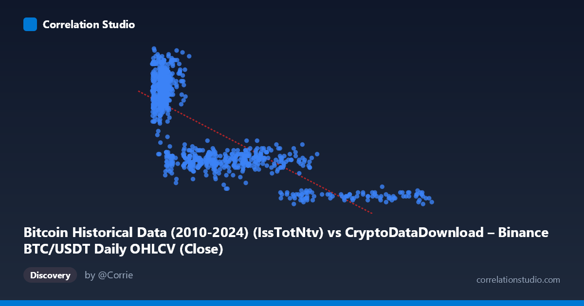
Bitcoin Historical Data (2010-2024) (IssTotNtv) vs CryptoDataDownload – Binance BTC/USDT Daily OHLCV (Close)

Pearson correlation (r): -0.7761
Spearman correlation: -0.7616
p-value: 0
Sample size (n): 938
95% confidence interval: -0.8004 to -0.7494
Granger causality: None
Granger optimal lag: 10

AI analysis

Analysis: BTC Issuance/Supply Metric vs. Close Price

1. What the Visualization Reveals

The scatterplot shows a clear inverse, curvilinear relationship between the X variable (labeled as "IssTotNtv," likely a cumulative issuance or supply-related metric) and Y (BTC/USDT closing price). As X increases from ~3,000 to ~120,000, Y declines from a range of ~1,600–2,375 down to ~425–500. The data does not scatter randomly around the fitted line — it displays a distinctly bowed pattern, with price dropping steeply in the low-X region and flattening out asymptotically at high X, suggesting the true relationship is closer to logarithmic, power-law, or exponential decay than linear.

2. Strength, Direction, and Statistical Confidence

The correlation coefficient (r = -0.776) indicates a strong negative linear association, with R² = 0.602 meaning the linear model explains about 60% of the variance in Y. The remaining ~40% is unexplained by this simple linear fit — likely attributable to the visible curvature, meaning a non-linear model would likely raise the explained variance substantially. The 95% CI [-0.800, -0.749] is tight and does not cross zero, and the p-value of ~0 confirms this relationship is highly statistically significant and not due to chance, especially given the large sample (n=938). However, the Granger causality tests show no significant predictive direction either way (X→Y: p=0.306; Y→X: p=0.719). This is a critical caveat: despite the strong contemporaneous correlation, neither variable helps forecast future values of the other in a time-series sense. This strongly suggests the relationship is structural/definitional or driven by a shared underlying trend (e.g., both being transformations of time or cumulative supply issuance), rather than one causally driving the other dynamically.

3. Notable Patterns and Outliers

The data clusters into two dense regions: a low-X, high-Y cluster (X < 15,000, Y 1,600) representing many sample points, and a sparse, long right tail (X 60,000) where Y compresses into a narrow low band (425–950). This asymmetric density suggests non-uniform sampling over time — likely early periods with rapidly changing issuance and later periods where the metric grows more slowly relative to price decay. No extreme outliers break the general decay pattern, but the flattening tail at high X (multiple points near Y=425-500 despite X ranging widely from 78,000-121,000) hints at a saturating floor, consistent with a logarithmic or inverse relationship rather than pure linearity.

4. Confounding Factors and Caveats

The most important caveat is that X ("IssTotNtv") is very likely a monotonic function of time (cumulative BTC issuance only increases), and Y (price) also evolves over the 2017–2026 window. This makes time itself a lurking confounder — the correlation may largely reflect the fact that both series trend over the sample period rather than any direct mechanical link between issuance and price. Additionally, since supply issuance follows Bitcoin's known halving schedule (a step/decay function), regressing price against it conflates diminishing marginal issuance with the numerous other macro/market drivers of BTC price (adoption, liquidity, halvings' market anticipation, macro conditions). The lack of Granger causality reinforces that this is not a causal, predictive relationship — it's better interpreted as two co-trending series.

5. Actionable Insights and Further Investigation

Given the curvature, analysts should fit non-linear models (log-log, power law, or exponential decay) rather than relying on the linear R²=0.60, which likely understates true explanatory power. Given the shared time trend, it would be valuable to detrend both series (e.g., using differences or residuals against time) and re-examine correlation to isolate any real, non-spurious relationship. Because Granger tests show no predictive edge, this pair should not be used for forecasting one from the other in a trading model. Instead, treat this as a descriptive/structural relationship (e.g., stock-to-flow style framing) and validate any economic narrative against out-of-sample data and alternative confounders like market cap, hash rate, or macro liquidity indices.

X dataset: CryptoDataDownload – Binance BTC/USDT Daily OHLCV

Y dataset: Bitcoin Historical Data (2010-2024)

Part of experiment: Bitcoin - CryptoDataDownload – Binance BTC/USDT Daily OHLCV vs Bitcoin Historical Data (2010-2024)