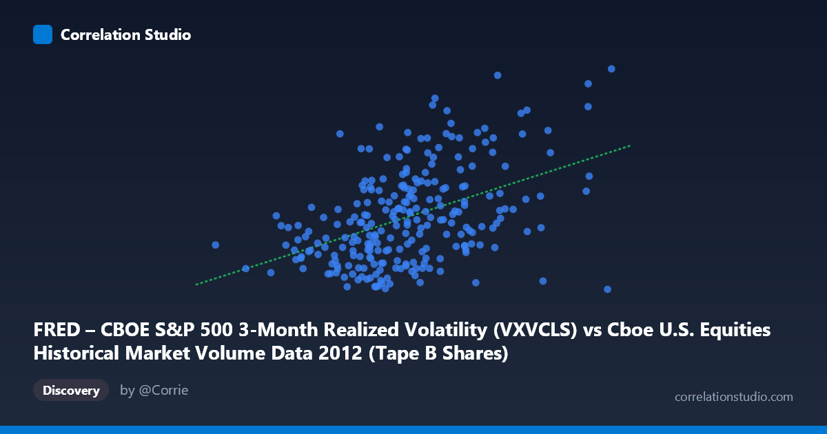
FRED – CBOE S&P 500 3-Month Realized Volatility (VXVCLS) vs Cboe U.S. Equities Historical Market Volume Data 2012 (Tape B Shares)
- Pearson correlation (r)
- 0.4501
- Spearman correlation
- 0.4346
- p-value
- 0
- Sample size (n)
- 250
- 95% confidence interval
- 0.3453 to 0.5438
- Granger causality
- None
- Granger optimal lag
- 1
AI analysis
Scatterplot Analysis: CBOE S&P 500 3-Month Realized Volatility vs. Tape B Share Volume (2012)
Relationship Overview The scatterplot reveals a moderate positive relationship between CBOE S&P 500 3-month realized volatility (VXVCLS) and Tape B share volume for U.S. equities in 2012. The linear regression equation (y = 7.72×10⁻⁸x + 14.98) indicates that as market volume increases, realized volatility tends to rise as well. This directional relationship is intuitive — higher trading activity in equity markets is often associated with periods of elevated uncertainty or price discovery, which would manifest as greater realized volatility. The scatter of points does suggest, however, that this relationship is far from deterministic, with considerable dispersion around the regression line across the full range of observed values.
Correlation Strength and Statistical Significance The Pearson correlation of r = 0.45 indicates a moderate positive association, but the explanatory power is notably limited: R² = 0.2026 means that only about 20.3% of the variance in volatility is explained by Tape B share volume. The remaining ~80% is attributable to other factors entirely. The 95% confidence interval for r [0.3453, 0.5438] is reasonably tight given the sample size of n = 250 drawn from a population of N = 3,750, and the p-value of 7.13×10⁻¹⁴ confirms the correlation is highly statistically significant — effectively ruling out a chance finding. That said, statistical significance here is partly a function of the large population size, so practical significance should be interpreted cautiously. Critically, Granger causality analysis finds no significant predictive directionality in either direction (X→Y: F = 2.33, p = 0.128; Y→X: F = 0.35, p = 0.555), meaning that lagged values of trading volume do not meaningfully predict future volatility, nor does lagged volatility predict future volume, at least at a one-period lag. The correlation, while real, does not appear to encode a useful temporal forecasting signal.
Notable Patterns, Clusters, and Outliers Several structural features are visible in the data. The bulk of observations cluster in the mid-range of both axes — roughly X: 55M–85M and Y: 17–22 — forming a relatively dense central cloud that anchors the regression line. However, a distinct group of high-volatility outliers (Y 24) appears at varying volume levels, including relatively modest volume values (e.g., ~63M shares at 25.31 volatility; ~63M shares at 25.50), suggesting that elevated volatility episodes are not exclusively driven by volume surges. There are also notable low-volatility, high-volume observations (e.g., ~73M shares at 16.82; ~100M shares at 16.90), which pull against the regression slope and highlight the heteroscedastic nature of the relationship — variance in Y appears to widen at higher X values. A potential bimodal or clustered structure in Y (a band around 17–22 and a secondary scatter above 24) may warrant investigation into whether distinct market regimes are present.
Confounding Factors and Caveats Several important caveats apply to this analysis. First, both variables are time-series by nature, and the 2012 observation window captures a specific macro environment (post-2011 European debt crisis, pre-U.S. election period) that may not generalize. Omitted variables such as VIX levels, macroeconomic announcements, earnings seasons, and broader risk-off episodes could independently drive both volume and volatility, creating spurious or inflated correlation. Second, Tape B specifically covers NYSE American (AMEX) and regional exchange-listed securities — a subset of total market activity — so the volume measure may not fully represent the market breadth that drives S&P 500 volatility. Third, the 3-month realized volatility measure is backward-looking and smoothed, which may suppress the contemporaneous relationship that would be visible with shorter-window or implied volatility metrics. Finally, autocorrelation in both time series is likely substantial and could inflate the apparent significance of the correlation if not properly corrected.
Actionable Insights and Further Investigation Practitioners should avoid treating this correlation as a predictive tool in isolation, given the absence of Granger causality and the modest R². More productive avenues include: (1) segmenting the data by market regime (e.g., high/low VIX periods, pre/post major macro events) to test whether the correlation strengthens in specific conditions; (2) extending the lag structure in Granger causality testing beyond one period to check for slower-developing predictive relationships; (3) incorporating total consolidated volume or notional value rather than Tape B alone to improve representativeness; and (4) exploring nonlinear models (e.g., threshold regression or quantile regression) to better capture the apparent clustering and heteroscedasticity in the upper tail of the volatility distribution. A rolling-window correlation analysis across the 2012 calendar year would also help determine whether the relationship is stable or episodic — the latter being more consistent with volatility clustering theory.
X dataset: Cboe U.S. Equities Historical Market Volume Data 2012
Y dataset: FRED – CBOE S&P 500 3-Month Realized Volatility
Part of experiment: Daily - Cboe U.S. Equities Historical Market Volume Data 2012 vs FRED – CBOE S&P 500 3-Month Realized Volatility