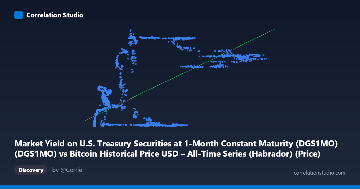
Market Yield on U.S. Treasury Securities at 1-Month Constant Maturity (DGS1MO) (DGS1MO) vs Bitcoin Historical Price USD – All-Time Series (Habrador) (Price)
- Pearson correlation (r)
- 0.6654
- Spearman correlation
- 0.6393
- p-value
- 0
- Sample size (n)
- 3946
- 95% confidence interval
- 0.6477 to 0.6825
- Granger causality
- None
- Granger optimal lag
- 1
- Time coverage
- 2010-07-19 to 2026-04-28
- Recomputed on refreshed data
- 2026-10-23 (r was 0.6654)
AI analysis
Analysis: Bitcoin Price vs. 1-Month Treasury Yield
Note on axis labeling: The metadata appears swapped — the values described as "X" (ranging 0.05–124,720) are clearly Bitcoin prices in USD, while "Y" (ranging 0.00–6.02) are Treasury yields in percent. The analysis below treats the data as it actually behaves: Treasury yield (0–6%) plotted against Bitcoin price ($0.05–$124,720).
1. What the Visualization Reveals The scatter shows a positive, non-linear association: as Bitcoin's price climbs from cents into the tens of thousands of dollars, the 1-month T-bill yield tends to be higher as well. At low BTC prices (under ~$1,000), yields cluster near zero (0.01–0.4%), consistent with the near-zero interest rate environment of 2010–2015 and again 2020–2021. Once BTC prices push into the $5,000–$125,000 range, yields become bimodal — some points still near zero, others clustering around 4–5.5%, reflecting the 2022–2024 Fed hiking cycle that coincided with BTC's later bull runs.
2. Strength, Direction, and Uncertainty The correlation (r = 0.665, R² = 0.443) indicates a moderate-to-strong positive linear relationship, with Treasury yield levels explaining about 44% of the variance in Bitcoin price (or vice versa, statistically). The 95% CI [0.648, 0.683] is tight and the p-value is effectively 0, so the correlation is highly statistically reliable — this is not sampling noise. However, statistical significance ≠ practical causal linkage: Granger causality tests show no significant predictive relationship in either direction (X→Y: p=0.39; Y→X: p=0.48). This is a critical finding: despite the strong contemporaneous correlation, neither series helps forecast the other's future values. This strongly suggests the relationship is spurious or driven by a shared external trend (e.g., both series reflect the passage of calendar time / macro regime) rather than genuine causal interaction.
3. Patterns, Clusters, and Outliers Three distinct clusters emerge: (a) a dense low-BTC/low-yield cluster (BTC < $1,000, yield < 0.3%) representing Bitcoin's early years under ZIRP; (b) a mid-range cluster (BTC $5,000–$19,000, yield 1–2.5%) corresponding to 2018–2019; and (c) a high-BTC/high-yield cluster (BTC $56,000–$125,000, yield 4–5.5%) matching 2023–2025. Notably, some high-BTC points still show near-zero yields (e.g., $34,574 → 0.05%; $40,162 → 0.02%), reflecting 2020–2021 when BTC rallied hard during zero-rate QE — these are the clearest deviations from the linear trend and pull R² down, evidencing the relationship's non-stationarity across regimes.
4. Confounding Factors and Caveats This is a classic time-series confound: both variables are trending over the same 15-year window, and simple correlation between two non-stationary trending series is prone to spurious inflation (a well-known econometric pitfall). The true driver is likely macroeconomic regime — Fed policy cycles (ZIRP era vs. hiking cycle) — which independently pushed yields up post-2022 while a separate set of factors (institutional adoption, ETF approval, halving cycles) pushed BTC prices up. The lack of Granger causality reinforces that this is correlation without a demonstrable lead-lag causal mechanism. Additionally, the linear R² (0.44) is likely understated/overstated depending on transformation — BTC price is extremely right-skewed (mean $20,782 vs. median likely far lower), so a log-transform of BTC price would probably fit the yield relationship (or lack thereof) more appropriately.
5. Suggestions for Further Investigation - Test for cointegration/stationarity (ADF tests, then a proper cointegration test) rather than relying on raw Pearson r, given both series trend over time. - Log-transform BTC price before correlating, since its distribution spans 6 orders of magnitude. - Detrend or difference both series (e.g., use % changes/returns rather than levels) and re-run correlation and Granger tests — this often eliminates spurious level-correlations in trending macro series. - Segment by monetary regime (ZIRP 2010–2021 vs. hiking 2022+) to check if the correlation reverses sign or disappears within-regime, which would confirm the relationship is regime-driven rather than a genuine yield→BTC or BTC→yield linkage.
X dataset: Bitcoin Historical Price USD – All-Time Series (Habrador)
Y dataset: Market Yield on U.S. Treasury Securities at 1-Month Constant Maturity (DGS1MO)
Part of experiment: Bitcoin - Bitcoin Historical Price USD – All-Time Series (Habrador) vs Market Yield on U.S. Treasury Securities at 1-Month Constant Maturity (DGS1MO)