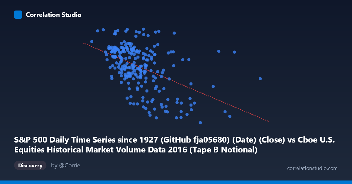
S&P 500 Daily Time Series since 1927 (GitHub fja05680) (Date) (Close) vs Cboe U.S. Equities Historical Market Volume Data 2016 (Tape B Notional)

Pearson correlation (r): -0.4865
Spearman correlation: -0.4684
p-value: 0
Sample size (n): 252
95% confidence interval: -0.5755 to -0.3861
Granger causality: None
Granger optimal lag: 1

AI analysis

Scatterplot Analysis: S&P 500 Close Price vs. Tape B Notional Trading Volume (2016)

Relationship Overview

The scatterplot reveals a moderate negative relationship between the S&P 500 daily closing price (X-axis) and Cboe Tape B notional trading volume (Y-axis) across the 2016 trading year. As S&P 500 prices increase, Tape B notional volume tends to decrease, and vice versa. This inverse pattern is visually apparent in the downward-sloping regression line (y = -3.16×10⁻⁸x + 2254.22), which cuts across a notably dispersed cloud of points. The data spans a wide X range (~2.05B to ~12.72B, though most observations cluster between ~3.5B and ~6.5B), while Y values remain relatively compressed between roughly 1,830 and 2,272 — suggesting Tape B notional volume is bounded within a fairly stable range despite considerable price variation.

Correlation Strength and Statistical Significance

The Pearson correlation of r = -0.487 indicates a moderate negative association, but the variance explained metric provides crucial perspective: r² = 0.237, meaning only about 23.7% of the variance in Tape B notional volume is accounted for by S&P 500 closing price. The remaining ~76% of variation is driven by factors outside this bivariate relationship. The 95% confidence interval of [-0.576, -0.386] is entirely negative and reasonably tight, confirming directional consistency, while the p-value of 2.22×10⁻¹⁶ — far below any conventional significance threshold — establishes that this correlation is extraordinarily unlikely to be a chance artifact given n = 252 paired observations drawn from a population of N = 3,622. However, statistical significance here should not be conflated with practical or economic importance; the modest r² tempers enthusiasm considerably. Critically, the Granger causality tests return no significant predictive direction in either direction (X→Y: F = 0.517, p = 0.473; Y→X: F = 0.092, p = 0.762), meaning neither variable meaningfully predicts the other's next-period value at the optimal lag of 1. The relationship, while real in a contemporaneous correlational sense, carries no demonstrated temporal predictive utility.

Notable Patterns, Clusters, and Outliers

The bulk of observations form a dense central cluster at mid-range X values (~3.5B–5.5B) and Y values (~2,050–2,200), consistent with the mean values reported. However, several notable outliers pull attention toward the extremes. A small group of points at very high X values (~8B–12.7B) tend to coincide with lower Y values (1,870–1,940), consistent with the negative trend but sitting far from the main cluster — these could represent unusual high-volume days or data anomalies worth scrutinizing. Conversely, one conspicuous point near x ≈ 6.3B achieves one of the highest Y values (~2,262), bucking the negative trend. There is also a suggestion of heteroscedasticity: variance in Y appears somewhat wider at lower X values and tighter at higher X values, which could partially reflect market regime differences earlier in 2016 (higher volatility period in January–February) versus more stable conditions later. No strong non-linear curvature is visually apparent, but the scatter is substantial enough that a linear model is a simplification.

Confounding Factors and Interpretive Caveats

Several important caveats apply. First, this is a temporal dataset (daily observations across one calendar year), meaning sequential data points are not independent — autocorrelation within each series is probable, which can inflate apparent correlations and violate OLS regression assumptions. Second, the axis labels appear swapped in the dataset metadata (Close price is labeled as X from the Cboe dataset, and Tape B Notional is labeled as Y from the S&P 500 dataset), suggesting a potential data join or labeling issue that should be verified before drawing firm conclusions. Third, market structure dynamics are a meaningful confounder: early 2016 saw significant market volatility and a sharp correction (S&P 500 prices were lower), which typically drives higher trading volumes — this cyclical volatility-volume relationship could explain much of the observed negative correlation without implying any direct causal mechanism between price level and Tape B specifically. Fourth, Tape B covers NYSE Arca-listed securities (primarily ETFs), whose volume dynamics may respond differently to market conditions than the broader S&P 500 price level implies.

Actionable Insights and Further Investigation

Given the moderate but incomplete explanatory power and the absence of Granger causality, practitioners should resist using S&P 500 price levels as a standalone predictor of Tape B notional volume. Instead, further investigation should explore: (1) incorporating implied volatility (VIX) as a covariate, since fear/volatility is a more theoretically grounded driver of trading activity than price level per se; (2) decomposing the time series to separate trend, seasonality, and noise before correlating, which would clarify whether the relationship persists after removing shared temporal drift; (3) testing lagged relationships beyond lag-1, as market structure effects may operate on weekly rather than daily cycles; and (4) verifying and correcting the apparent dataset labeling inconsistency to ensure the axes represent what they claim. A multivariate model including VIX, day-of-week effects, and macro event indicators would likely substantially improve on the current 23.7% explained variance.

X dataset: Cboe U.S. Equities Historical Market Volume Data 2016

Y dataset: S&P 500 Daily Time Series since 1927 (GitHub fja05680) (Date)

Part of experiment: Daily - Cboe U.S. Equities Historical Market Volume Data 2016 vs S&P 500 Daily Time Series since 1927 (GitHub fja05680) (Date)